Preparation of Input Data

To characterize a flow system, users need to prepare input data, including hydrogeologic and thermal parameters and constitutive relations of the permeable medium (absolute and relative permeability, porosity, capillary pressure, heat conductivity, etc.), thermophysical properties of the fluids (mostly provided internally), initial and boundary conditions of the flow system, and sinks and sources. In addition, TOUGH3 requires specification of space-discretized geometry, and various program options, computational parameters, and time-stepping information. Here we summarize the basic conventions adopted for TOUGH3 input data (Section TOUGH3 Input Data), and provide a detailed explanation of input data formats (Section TOUGH3 Input Format); the summary and input formats for internal grid generation through the MESHMaker module are explained in Sections Geometry Data and Input Formats for MESHMAKER, respectively. Some of the EOS modules have specialized input requirements (discussed in the addenda for those modules). The TMVOC, ECO2N, and ECO2M modules have special options and input requirements, which are explained in separate reports (TMVOC: Pruess and Battistelli, 2002; ECO2N: Pruess, 2005, Pan et al., 2015; ECO2M: Pruess, 2013).

TOUGH3 Input Data

Input can be provided to TOUGH3 in a flexible manner by means of one or several ASCII data files. All TOUGH3 input is in fixed format (a few exceptions, such as data blocks GENER and TIMBC) and standard metric (SI) units, such as meters, seconds, kilograms, ˚C, and the corresponding derived units, such as Newtons, Joules, and Pascal = N/m² for pressure.

In the standard TOUGH3 input file data are organized in blocks which are defined by five-character keywords typed in columns 1-5; see Table 2. The first record must be a problem title of up to 80 characters. The last record usually is ENDCY; alternatively, ENDFI may be used if no flow simulation is to be carried out (useful for mesh generation). Data records beyond ENDCY (or ENDFI) will be ignored. Some data blocks, such as those specifying reservoir domains (ROCKS), volume elements (ELEME), connections (CONNE), sinks/sources (GENER), and initial conditions (INDOM and INCON), have a variable number of records, while others have a fixed number of records. The end of variable-length data blocks is indicated by a blank record. The data blocks can be provided in arbitrary order; exceptions are (1) the first line must be the title line, (2) ELEME, if present, must precede CONNE, (3) START, if present, must be specified before INCON, and (4) MULTI must be specified before PARAM, INDOM, INCON (only if \(NKIN \ne NK\)), and OUTPU. The blocks ELEME and CONNE must either be both provided through the input file, or must both be absent, in which case alternative means for specifying geometry data will be employed (see Section Geometry Data). If START is present, the block INCON can be incomplete, with elements in arbitrary order, or can be absent altogether. Elements for which no initial conditions are specified in INCON will then be assigned domain-specific initial conditions from block INDOM, if present, or will be assigned default initial conditions given in block PARAM, along with default porosities given in ROCKS. If START is not present, INCON must contain information for all elements, in exactly the same order as they are listed in block ELEME (note that initial conditions will be assigned to elements according to their order, not the element name).

Table 2 TOUGH3 input data blocks.

Keyword	Function
TITLE	first record, single line with a title for the simulation problem
MESHM	parameters for internal grid generation through MESHMaker
ROCKS	hydrogeologic parameters for various reservoir domains
MULTI	specifies number of fluid components and balance equations per grid block
SELEC	used with certain EOS-modules to supply thermophysical property data
START	one data record for more flexible initialization
PARAM	computational parameters; time stepping and convergence parameters; program options; default initial conditions
MOMOP	more program options
SOLVR	parameters for linear equation solver
DIFFU	diffusivities of mass components
FOFT	specifies grid blocks for which time series data are desired
COFT	specifies connections for which time series data are desired
GOFT	specifies sinks/sources for which time series data are desired
RPCAP	parameters for relative permeability and capillary pressure functions
HYSTE	parameters for hysteretic characteristic curves; required only if non-default values of parameters are used
TIMES	specification of times for generating printout
ELEME*	list of grid blocks (volume elements)
CONNE*	list of flow connections between grid blocks
GENER*	list of mass or heat sinks and sources
INDOM	list of initial conditions for specific reservoir domains
INCON*	list of initial conditions for specific grid blocks
TIMBC	specifies time-dependent Dirichlet boundary conditions
OUTPU	specifies variables/parameters for printout
ENDCY	last record to close the TOUGH3 input file and initiate the simulation
ENDFI	alternative to ENDCY for closing a TOUGH3 input file; will cause flow simulation to be skipped; useful if only mesh generation is desired

Note

* These blocks can be provided on separate disk files, in which case they would be omitted from the INPUT file.

Between data blocks, an arbitrary number of records with arbitrary data may be present that do not begin with any of the TOUGH3 keywords. This is useful for inserting comments about problem specifications directly into the input file. TOUGH3 will gather all these comments and will print the first 50 such records in the output file.

Much of the data handling in TOUGH3 is accomplished by means of disk files, which are written in a format of 80 characters per record, so that they can be edited and modified with any text editor.

Table 3 summarizes the disk files other than (default) INPUT and OUTPUT used in TOUGH3. The initialization of the arrays for geometry, generation, and initial condition data is always made from the disk files MESH (or MINC), GENER, and INCON. A user can either provide these files at execution time, or they can be written from TOUGH3 input data during the initialization phase of the program. During this initialization phase, two binary files MESHA and MESHB are created from the disk file MESH. If MESHA and MESHB exist in the working folder, the code will ignore the MESH file and the ELEME and CONNE blocks in the input file, and read geometric information directly from these two files, which will reduce the memory requirement for the master processor and enhance I/O efficiency. If the mesh is changed, MESHA and MESHB must be deleted from the working folder to make the changes take effect. If no data blocks GENER and INCON are provided in the input file, and if no disk files GENER and INCON are present, defaults will take effect (no generation; domain-specific initial conditions from block INDOM, or defaults from block PARAM). If a user intends to use these defaults, the user has to make sure that at execution time no disk files INCON or GENER are present from a previous run (or perhaps from a different problem). A safe way to use default GENER and INCON is to specify “dummy” data blocks in the input file, consisting of one record with GENER or INCON, followed by a blank record.

The format of data blocks ELEME, CONNE, GENER, and INCON is basically the same when these data are provided as disk files as when they are given as part of the input file. However, specification of these data through the input file rather than as disk files offers some added conveniences, which are useful when a new simulation problem is initiated. For example, a sequence of identical items (volume elements, connections, sinks or sources) can be specified through a single data record. Also, indices used internally for cross-referencing elements, connections, and sources will be generated internally by TOUGH3 rather than having them provided by the user. MESH, GENER, and INCON disk files written by TOUGH3 can be merged into an input file without changes, keeping the cross-referencing information.

Table 3 TOUGH3 disk files.

File	Use
MESH	written in subroutine INPUT from ELEME and CONNE data, or in module MESHMaker from mesh specification data; read in RFILE to initialize all geometry data arrays used to define the discretized flow problem
GENER	written in subroutine INPUT from GENER data; read in RFILE to define nature, strength, and time-dependence of sinks and sources
INCON	written in subroutine INPUT from INCON data; read in RFILE to provide a complete specification of initial thermodynamic conditions
SAVE	written in subroutine WRIFI to record thermodynamic conditions at the end of a TOUGH3 simulation run; compatible with formats of file or data block INCON for initializing a continuation run
MINC	written in module MESHMaker with MESH-compatible specifications, to provide all geometry data for a fractured-porous medium mesh (double porosity, dual permeability, multiple interacting continua); read (optionally) in subroutine RFILE to initialize geometry data for a fractured-porous system
TABLE	written in subroutine CYCIT to record coefficients of semi-analytical linear heat exchange with confining beds at the end of a TOUGH3 simulation run; read (optionally) in subroutine QLOSS to initialize heat exchange coefficients in a continuation run

TOUGH3 Input Format

Here we cover the common input data for all EOS modules of TOUGH3. Additional EOS-specific input data are discussed in the addendum for each EOS module. The format described is for the default five-character element names.

TITLE

This is the first record of the input file, containing a header of up to 80 characters, to be printed on output. This can be used to identify a problem. If no title is desired, leave this record blank.

ROCKS

Introduces material parameters for different reservoir domains.

Table 4 Record ROCKS.1.

Parameter	Format	Description
MAT	A5	material name (rock type).
NAD	I5	if zero or negative, defaults will take effect for a number of parameters (see below): ≥ 1: will read another data record to override defaults. ≥ 2: will read two more records with domain-specific parameters for relative permeability and capillary pressure functions.
DROK	E10.4	rock grain density (kg/m3`). If DROK is set to a very large value (typically 1.0E50), a constant temperature boundary condition can be specified (but variable pressure/saturation).
POR	E10.4	default porosity (void fraction) for all elements belonging to domain MAT for which no other porosity has been specified in block INCON. Option START is necessary for using default porosity.
PER(I)	E10.4	I = 1, 3 absolute permeabilities along the three principal axes, as specified by ISOT in block CONNE.
CWET	E10.4	formation heat conductivity under fully liquid-saturated conditions (W/m ˚C).
SPHT	E10.4	rock grain specific heat (J/kg ˚C). Domains with SPHT > 104 J/kg ˚C will not be included in global material balances. This provision is useful for boundary nodes, which are given very large volumes so that their thermo-dynamic state remains constant. Because of the large volume, inclusion of such nodes in global material balances would make the balances useless.

When a (dummy) domain named “SEED” is specified, the absolute permeabilities specified in PER(I) are modified by the block-by-block permeability modifiers (PM) according to:

(45)\[k_n \rightarrow k_n^{'} = k_n \cdot \zeta_n\]

Here, \(k_n\) is the absolute (“reference”) permeability of grid block \(n\), as specified in data block ROCKS for the domain to which that grid block belongs, \(k_n^{'}\) is the modified permeability, and \(\zeta_n\) is the PM coefficient. When PM is in effect, the strength of capillary pressure will be automatically scaled according to (Leverett, 1941)

(46)\[P_{cap, n} \rightarrow P_{cap, n}^{'} = \frac{P_{cap, n}}{\sqrt{\zeta_n}}\]

No grid blocks should be assigned to this domain; the presence of domain “SEED” simply serves as a flag to put permeability modification into effect. Random (spatially uncorrelated) PM data can be internally generated in TOUGH3. Alternatively, externally defined permeability modifiers may be provided as part of the geometry data (PMX) in block ELEME. Available PM options are:

1. Externally supplied: \(\zeta_n = PMX - PER(2)\)

2. “Linear”: \(\zeta_n = PER(1) \times s - PER(2)\)

3. “Logarithmic”: \(\zeta_n = \exp \left( - PER(1) \times s \right) - PER(2)\)

where \(s\) is a random number between 0 and 1.

Data provided in domain “SEED” are used to select the following options.

Table 5 Domain “SEED”.

Parameter	Format	Description
DROK	E10.4	random number seed for internal generation of “linear” permeability modifiers: = 0: (default) no internal generation of “linear” permeability modifiers. > 0: perform “linear” permeability modification; random modifiers are generated internally with DROK as seed.
POR	E10.4	random number seed for internal generation of “logarithmic” permeability modifiers: = 0: (default) no internal generation of “logarithmic” permeability modifiers. > 0: perform “logarithmic” permeability modification; random modifiers are generated internally with POR as seed.
PER(1)	E10.4	scale factor (optional) for internally generated permeability modifiers: = 0: (defaults to PER(1) = 1): permeability modifiers are generated as random numbers in the interval (0, 1). > 0: permeability modifiers are generated as random numbers in the interval (0, PER(1)).
PER(2)	E10.4	shift (optional) for internal or external permeability modifiers: = 0: (default) no shift is applied to permeability modifiers. > 0: permeability modifiers are shifted according to \(\zeta_n^{'} = \zeta_n - PER(2)\). All \(\zeta_n^{'} \lt 0\) are set equal to zero.

If both DROK and POR are specified as non-zero, DROK takes precedence. And if both DROK and POR are zero, permeability modifiers as supplied through ELEME data will be used. Note that the domain “SEED” is not required in TOUGH3 if externally defined permeability modifiers in block ELEME are used without any shift.

Table 6 Record ROCKS.1.1 (optional, NAD ≥ 1 only).

Parameter	Format	Description
COM	E10.4	pore compressiblity (Pa-1), \(\frac{1}{\phi} \left( \frac{\partial \phi}{\partial P} \right)_T\), (default is 0).
EXPAN	E10.4	pore expansivity (1/ ˚C), \(\frac{1}{\phi} \left( \frac{\partial \phi}{\partial T} \right)_P\), (default is 0).
CDRY	E10.4	formation heat conductivity under desaturated conditions (W/m ˚C), (default is CWET).
TORTX	E10.4	tortuosity factor for binary diffusion. If TORTX = 0, a porosity and saturation-dependent tortuosity will be calculated internally from the Millington & Quirk, 1961 model, Eq. (12). When diffusivities, FDDIAGin data block DIFFU, are specified as negative numbers, \(\tau_0 \tau_{\beta} = S_{\beta}\) will be used.
GK	E10.4	Klinkenberg parameter b (Pa-1`) for enhancing gas phase permeability according to the relationship \(k_{gas} = k \left( 1 + \frac{b}{P} \right)\).
XKD3	E10.4	Distribution coefficient for parent radionuclide, Component 3, in the aqueous phase, m3` kg-1 (EOS7R only).
XKD4	E10.4	Distribution coefficient for daughter radionuclide, Component 4, in the aqueous phase, m3` kg-1 (EOS7R only).

Table 7 Record ROCKS.1.2 (optional, NAD ≥ 2 only).

Parameter	Format	Description
IRP	I5	integer parameter to choose type of relative permeability function.
	5X	(void)
RP(I)	E10.4	I = 1, …, 7 parameters for relative permeability function.

Table 8 Record ROCKS.1.2.1 (optional, IRP = 12 only).

Parameter	Format	Description
RP(I)	E10.4	I = 8, …, 10 parameters for relative permeability function.

Table 9 Record ROCKS.1.3 (optional, NAD ≥ 2 only).

Parameter	Format	Description
ICP	I5	integer parameter to choose type of capillary pressure function.
	5X	(void)
CP(I)	E10.4	I = 1, …, 7 parameters for capillary pressure function.

Table 10 Record ROCKS.1.3.1 (optional, ICP = 12 only).

Parameter	Format	Description
CP(I)	E10.4	I = 8, …, 13 parameters for capillary pressure function.

Repeat records 1, 1.1, 1.2, 1.2.1., 1.3, and 1.3.1 for different reservoir domains.

A blank record closes the ROCKS data block.

MULTI

Permits the user to select the number and nature of balance equations that will be solved. For most EOS modules this data block is not needed, as default values are provided internally. Available parameter choices are different for different EOS modules (see the addendum of the EOS module of interest).

Table 11 Record MULTI.1.

Parameter	Format	Description
NK	I5	number of mass components.
NEQ	I5	number of balance equations per grid block. Usually we have NEQ = NK + 1, for solving NK mass and one energy balance equation. Some EOS modules allow the option NEQ = NK, in which case only NK mass balances and no energy equation will be solved.
NPH	I5	number of phases that can be present (2 for most EOS modules).
NB	I5	number of secondary parameters in the PAR-array other than component mass fractions. Available options include NB = 6 (no diffusion) and NB = 8 (include diffusion).
NKIN	I5	number of mass components in INCON data (default is NKIN = NK). This parameter can be used, for example, to initialize an EOS7R simulation (NK = 4 or 5) from data generated by EOS7 (NK = 2 or 3). If a value other than the default is to be used, then data block MULTI must appear before any initial conditions in data blocks PARAM, INDOM, or INCON.

START (optional)

A record with START typed in columns 1-5 allows a more flexible initialization. More specifically, when START is present, INCON data can be in arbitrary order, and need not be present for all grid blocks (in which case defaults will be used). Without START, there must be a one-to-one correspondence between the data in blocks ELEME and INCON.

PARAM

Introduces computation parameters, time stepping information, and default initial conditions.

Table 12 Record PARAM.1.

Parameter	Format	Description
NOITE	I2	specifies the maximum number of Newtonian iterations per time step (default is 8).
KDATA	I2	specifies amount of printout (default is 1): 0 or 1: print a selection of element variables. 2: in addition, print a selection of connection variables. 3: in addition, print a selection of generation variables. If the above values for KDATA are increased by 10, printout will occur after each Newton-Raphson iteration (not just after convergence). If negative values are used, printout for the selection of variables will be generated in the file format of TECPLOT. The amount of printout is given by the absolute value of KDATA.
MCYC	I4	maximum number of time steps to be calculated. If a negative value is used, MCYC = 2-MCYC.
MSEC	I4	maximum duration, in CPU seconds, of the simulation (default is infinite).
MCYPR	I4	printout will occur for every multiple of MCYPR steps (default is 1). If a negative value is used, MCYPR = 2-MCYPR.
MOP(I)	I1	I = 1, 24 allows choice of various options, which are documented in printed output from a TOUGH3 run.
MOP(1)	I1	if unequal 0, a short printout for non-convergent iterations will be generated.
MOP(2) … MOP(6)	I1	generate additional printout in various sub-routines, if set unequal 0. This feature should not be needed in normal applications, but it will be convenient when a user suspects a bug and wishes to examine the inner workings of the code. The amount of printout increases with MOP(I) (consult source code listings for details).
MOP(2)	I1	CYCIT (main subroutine).
MOP(3)	I1	MULTI (flow- and accumulation-terms).
MOP(4)	I1	QU (sinks/sources). No longer supported in TOUGH3.
MOP(5)	I1	EOS (equation of state).
MOP(6)	I1	LINEQ (linear equations). No longer supported in TOUGH3.
MOP(7)	I1	if unequal 0, a printout of input data will be provided.
MOP(8)	I1	if ISOT < 0, chooses the option for reducing fracture-matrix interface area.
MOP(9)	I1	determines the composition of produced fluid with the MASS option (see GENER). The relative amounts of phases are determined as follows: 0: according to relative mobilities in the source element. 1: produced source fluid has the same phase composition as the producing element.
MOP(10)	I1	chooses the interpolation formula for heat conductivity as a function of liquid saturation (\(S_l\)): 0: \(C(S_l) = CDRY + \sqrt{S_l} \left( CWET - CDRY \right)\). 1: \(C(S_l) = CDRY + S_l \left( CWET - CDRY \right)\).
MOP(11)	I1	determines evaluation of mobility and permeability at interfaces: 0: mobilities are upstream weighted with WUP (see PARAM.3), permeability is upstream weighted. 1: mobilities are averaged between adjacent elements, permeability is upstream weighted. 2: mobilities are upstream weighted, permeability is harmonic weighted. 3: mobilities are averaged between adjacent elements, permeability is harmonic weighted. 4: mobility and permeability are both harmonic weighted.
MOP(12)	I1	determines interpolation procedure for time dependent sink/source data (flow rates and enthalpies): 0: triple linear interpolation; tabular data are used to obtain interpolated rates and enthalpies for the beginning and end of the time step; the average of these values is then used. 1: step function option; rates and enthalpies are taken as averages of the table values corresponding to the beginning and end of the time step. 2: rigorous step rate capability for time dependent generation data. A set of times \(t_i\) and generation rates \(q_i\) provided in data block GENER is interpreted to mean that sink/source rates are piecewise constant and change in discontinuous fashion at table points. Specifically, generation is assumed to occur at constant rate \(q_i\) during the time interval \([t_i, t_{i+1})\), and changes to \(q_{i+1}\) at \(t_{i+1}\). Actual rate used during a time step that ends at time \(t\), with \(t_i \le t \le t_{i+1}\), is automatically adjusted in such a way that total cumulative exchanged mass at time \(t\) (47)\[Q(t) = \int_0^t q dt^{'} = \sum_{j=1}^{i-1} q_j \left( t_{j+1} - t_j \right) + q \left( t - t_i \right)\] is rigorously conserved. If also tabular data for enthalpies are given, an analogous adjustment is made for fluid enthalpy, to preserve \(\int qh dt\).
MOP(13)	I1	determines content of INCON and SAVE files: 0: standard content. 1: writes user-specified initial conditions to file SAVE. 2: reads parameters of hysteresis model from file INCON.
MOP(14)	I1	(void)
MOP(15)	I1	determines conductive heat exchange with impermeable geologic formations using semi-analytical methods: 0: heat exchange is off. 1: linear heat exchange between a reservoir and confining beds is on (for grid blocks that have a non-zero heat transfer area; see data block ELEME). Initial temperature in cap- or base-rock is assumed uniform and taken as the temperature with which the last element in data block ELEME is initialized. 2: linear heat exchange between a reservoir and confining beds is on. Initial temperature for the confining bed adjacent to an element that has a non-zero heat transfer area is taken as the temperature of that element in data block INCON. Heat capacity and conductivity of the confining beds are specified in block ROCKS for the particular domain to which the very last volume element in data block ELEME belongs. Thus, if a semi-analytical heat exchange calculation is desired, the user would append an additional dummy element of a very large volume at the end of the ELEME block, and provide the desired parameters as initial conditions and domain data, respectively, for this element. It is necessary to specify which elements have an interface area with the confining beds, and to give the magnitude of this interface area. This information is input as parameter AHTX in columns 31-40 of volume element data in block ELEME. Volume elements for which a zero-interface area is specified will not be subject to heat exchange. A sample problem using MOP(15) = 1 is included in the addendum for EOS1. 5: radial heat exchange between fluids in a wellbore and the surrounding formation is on. Constant well and formation properties are given in a material named QLOSS with the following parameters: - DROK: Rock grain density [kg/m3] of formation near well - POR: Well radius [m] - PER(1): Reference elevation [m]; specify Z coordinate in block ELEME, columns 71-80 - PER(2): Reference temperature [˚C] - PER(3): Geothermal gradient [˚C/m] - CWET: Heat conductivity [W/kg ˚C] of formation near well - SPHT: Rock grain specific heat [J/kg ˚C] of formation near well 6: radial heat exchange between fluids in a wellbore and the surrounding formation is on. Depth-dependent well and formation properties (depth, radius, temperature, conductivity, density, capacity) are provided on an external file named radqloss.dat with the information in the following format: on the first line, NMATQLOSS is the number of elevations with geometric and thermal data, and NMATQLOSS lines are provided with the following data in free format: elevation [m], well radius [m], initial temperature [˚C], CWET, DROK, SPHT. Between elevations, properties are calculated using linear interpolation. RESTART is possible for linear heat exchange between a reservoir and confining beds (MOP(15) = 1 or 2), but not for radial heat exchange (MOP(15) = 5 or 6). The data necessary for continuing the linear heat exchange calculation in a TOUGH3 continuation run are written onto a disk file TABLE. When restarting a problem, this file has to be provided under the name TABLE. If file TABLE is absent, TOUGH3 assumes that no prior heat exchange with confining beds has taken place.
MOP(16)	I1	provides automatic time step control: 0: automatic time stepping based on maximum change in saturation. 1: automatic time stepping based on number of iterations needed for convergence. >1: time step size will be doubled if convergence occurs within ITER ≤ MOP(16) Newton-Raphson iterations. It is recommended to set MOP(16) in the range of 2-4.
MOP(17)	I1	handles time stepping after linear equation solver failure: 0: no time step reduction despite linear equation solver failure. 9: reduce time step after linear equation solver failure.
MOP(18)	I1	selects handling of interface density: 0: perform upstream weighting for interface density. >0: average interface density between the two grid blocks. However, when one of the two phase saturations is zero, upstream weighting will be performed.
MOP(19)	I1	switch used by different EOS modules for conversion of primary variables.
MOP(20)	I1	switch for vapor pressure lowering in EOS4; MOP(20) = 1 optionally suppresses vapor pressure lowering effects.
MOP(21)	I1	selects the linear equation solver: 0: defaults to MOP(21) = 3, DSLUCS, Lanczos-type preconditioned bi-conjugate gradient solver. 1: (void) 2: DSLUBC, bi-conjugate gradient solver. 3: DSLUCS (default). 4: DSLUGM, generalized minimum residual preconditioned conjugate gradient solver. 5: DLUSTB, stabilized bi-conjugate gradient solver. 6: LUBAND, banded direct solver. 7: AZTEC parallel iterative solver. 8: PETSc parallel iterative solver. All conjugate gradient solvers use incomplete LU-factorization as a default preconditioner. Other preconditioners may be chosen by means of a data block SOLVR.
MOP(22)	I1	(void)
MOP(23)	I1	(void)
MOP(24)	I1	determines handling of multiphase diffusive fluxes at interfaces: - 0: harmonic weighting of fully coupled effective multiphase diffusivity. - 1: separate harmonic weighting of gas and liquid phase diffusivities.
TEXP	E10.4	parameter for temperature dependence of gas phase diffusion coefficient (see Eq. (13)).
BE	E10.4	(optional) parameter for effective strength of enhanced vapor diffusion; if set to a non-zero value, will replace the parameter group \(\phi \tau_0 \tau_{\beta}\) for vapor diffusion (see Eq. (10)).

Table 13 Record PARAM.2.

Parameter	Format	Description
TSTART	E10.4	starting time of simulation in seconds (default is 0).
TIMAX	E10.4	time in seconds at which simulation should stop (default is infinite).
DELTEN	E10.4	length of time steps in seconds. If DELTEN is a negative integer, DELTEN = -NDLT, the program will proceed to read NDLT records with time step information. Note that -NDLT must be provided as a floating point number, with decimal point.
DELTMX	E10.4	upper limit for time step size in seconds (default is infinite).
ELST	A5	no longer supported in TOUGH3. For printout after each time step, use FOFT instead.
	5X	(void)
GF	E10.4	magnitude (m/s2) of the gravitational acceleration vector. Blank or zero gives “no gravity” calculation.
REDLT	E10.4	factor by which time step is reduced in case of convergence failure or other problems (default is 4).
SCALE	E10.4	scale factor to change the size of the mesh (default = 1.0).

Table 14 Record PARAM.2.1.

Parameter	Format	Description
DLT(I)	E10.4	Length (in seconds) of time step I. This set of records is optional for DELTEN = -NDLT, a negative integer. Up to 13 records can be read, each containing 8 time step data. If the number of simulated time steps exceeds the number of DLT(I), the simulation will continue with time steps determined by automatic time step control (MOP(16)).

Table 15 Record PARAM.3.

Parameter	Format	Description
RE1	E10.4	convergence criterion for relative error (default 10-5`).
RE2	E10.4	convergence criterion for absolute error (default 1).
U	E10.4	(void)
WUP	E10.4	upstream weighting factor for mobilities and enthalpies at interfaces (default 1.0 is recommended). 0 ≤ WUP ≤ 1.
WNR	E10.4	weighting factor for increments in Newton/Raphson - iteration (default 1.0 is recommended). 0 < WNR ≤ 1.
DFAC	E10.4	increment factor for numerically computing derivatives (default value is DFAC = 10-k/2, where \(k\), evaluated internally, is the number of significant digits of the floating point processor used; for 64-bit arithmetic, DFAC ≈ 10-8).
FOR	E10.4	factor to change the size of the time step during the Newtonian iteration (default 1.0).
AMRES	E10.4	maximum permissible residual during the Newtonian iteration. If a residual larger than AMRES is encountered, time step will automatically be reduced (default 105).

Table 16 Record PARAM.4.

Parameter	Format	Description
X(I)	E20.13	I = 1, NKIN + 1 primary variables which are used as default initial conditions for all grid blocks that are not assigned by means of data blocks INDOM or INCON. Option START is necessary to use default INCON. Different sets of primary variables are in use for different EOS modules.

The number of primary variables, NKIN + 1, is normally assigned internally in the EOS module, and is usually equal to the number NEQ of equations solved per grid block. See data block MULTI for special assignments of NKIN. When more than four primary variables are used more than one line (record) must be provided.

INDOM

Introduces domain-specific initial conditions. These will supersede default initial conditions specified in PARAM.4, and can be overwritten by element-specific initial conditions in data block INCON. Option START is needed to use INDOM conditions.

Table 17 Record INDOM.1.

Parameter	Format	Description
MAT	A5	name of a reservoir domain, as specified in data block ROCKS.

Table 18 Record INDOM.2.

Parameter	Format	Description
X(I)	E20.13	I = 1, NKIN + 1 primary variables assigned to all grid blocks in the domain specified in record INDOM.1. Different sets of primary variables are used for different EOS modules.

A blank record closes the INDOM data block. Repeat records INDOM.1 and INDOM.2 for as many domains as desired. The ordering is arbitrary and need not be the same as in block ROCKS.

INCON

Introduces element-specific initial conditions.

Table 19 Record INCON.1.

Parameter	Format	Description
EL, NE	A3, I2	code name of element.
NSEQ	I5	number of additional elements with the same initial conditions.
NADD	I5	increment between the code numbers of two successive elements with identical initial conditions.
PORX	E15.9	porosity; if zero or blank, porosity will be taken as specified in block ROCKS if option START is used.
USRX(I)	E10.4	I = 1, 5 grid block specific parameters (optional).

Table 20 Record INCON.2.

Parameter	Format	Description
X(I)	E20.14	I = 1, NKIN + 1 primary variables for the element specified in record INCON.1. INCON specifications will supersede default conditions specified in PARAM.4, and domain-specific conditions that may have been specified in data block INDOM. Different sets of primary variables are used for different EOS modules.

A blank record closes the INCON data block. Alternatively, initial condition information may terminate on a record with +++ typed in the first three columns, followed by time stepping information. This feature is used for a continuation run from a previous TOUGH3 simulation.

SOLVR (optional)

Introduces a data block with parameters for linear equation solvers. For the parallel solvers, only MATSLV is used, and the other options should be specified through the PETSc (.petscrc) and Aztec (.aztecrc) option files.

Table 21 Record SOLVR.1.

Parameter	Format	Description
MATSLV	I1	selects the linear equation solver: 1: (void) 2: DSLUBC, a bi-conjugate gradient solver 3: DSLUCS, a Lanczos-type bi-conjugate gradient solver 4: DSLUGM, a generalized minimum residual solver 5: DLUSTB, a stabilized bi-conjugate gradient solver 6: direct solver LUBAND 7: AZTEC parallel iterative solver 8: PETSc parallel iterative solver
	2X	(void)
ZPROCS	A2	selects the Z-preconditioning (Moridis & Pruess, 1998). Regardless of user specifications, Z-preprocessing will only be performed when iterative solvers are used (2 ≤ MATSLV ≤ 5), and if there are zeros on the main diagonal of the Jacobian matrix: Z0: no Z-preprocessing (default for NEQ = 1) Z1: replace zeros on the main diagonal by a small constant (10-25; default for NEQ ≠ 1) Z2: make linear combinations of equations for each grid block to achieve non-zeros on the main diagonal Z3: normalize equations, followed by Z2 Z4: affine transformation to unit main-diagonal submatrices, without center pivoting
	3X	(void)
OPROCS	A2	selects the O-preconditioning (Moridis & Pruess, 1998): O0: no O-preprocessing (default, also invoked for NEQ = 1) O1: eliminate lower half of the main-diagonal submatrix with center pivoting O2: O1, plus eliminate upper half of the main-diagonal submatrix with center pivoting O3: O2, plus normalize, resulting in unit main-diagonal submatrices O4: affine transformation to unit main-diagonal submatrices, without center pivoting
RITMAX	E10.4	selects the maximum number of CG iterations as a fraction of the total number of equations (0.0 < RITMAX ≤ 1.0; default is RITMAX = 0.1).
CLOSUR	E10.4	convergence criterion for the CG iterations (10-12 ≤ CLOSUR ≤ 10-6; default is CLOSUR = 10-6)

FOFT (optional)

Introduces a list of elements (grid blocks) for which time-dependent data are to be written out for plotting during the simulation. A separate file is generated for each element in CSV format. The name of each file starts with FOFT, and includes the element name. If regular or simple hysteresis is invoked via IRP = ICP = 12 or IRP = ICP = 13, then relevant hysteresis parameters are also written to FOFT. If MOP2(17) > 0, print variables according to the input data in block OUTPU.

Table 22 Record FOFT.1.

Parameter	Format	Description
EFOFT	A5	element name.
	5X	(void)
IFOFTF	I5	a flag to control the amount of printout: 0: default printout of pressure, temperature, and saturation of flowing phases. >0: print out mass fraction of each component in the specified phase in addition to the default printout. <0: print out mass fraction of each component in each of all the flowing phases in addition to the default printout.

A blank record closes the FOFT data block. Repeat records FOFT.1 for as many elements as desired.

COFT (optional)

Introduces a list of connections for which time-dependent data are to be written out for plotting during the simulation. A separate file is generated for each connection in CSV format. The name of each file starts with COFT, and includes the pair of two element names.

Table 23 Record COFT.1.

Parameter	Format	Description
ECOFT	A10	a connection name, i.e., an ordered pair of two element names (no blank between elements).
	10X	(void)
ICOFTF	I5	a flag to control the amount of printout: 0: default printout of heat flux and flow rate of each flowing phase. >0: print out fractional mass flow of each component in the specified phase in addition to the default printout. <0: print out fractional mass flow of each component in each of all the flowing phases in addition to the default printout.

A blank record closes the COFT data block. Repeat records COFT.1 for as many connections as desired.

GOFT (optional)

Introduces a list of sinks/sources for which time-dependent data are to be written out for plotting during the simulation. A separate file is generated for each sink/source in CSV format. The name of each file starts with GOFT, and includes the sink/source name.

Table 24 Record GOFT.1.

Parameter	Format	Description
EGOFT	A5	the name of an element in which a sink/source is defined.
	5X	(void)
IGOFTF	I5	a flag to control the amount of printout: 0: default printout of mass flow rate and flowing enthalpy. >0: print out fractional mass flow rate of the specified phase in addition to the default printout. <0: print out fractional mass flow rate of each of all the flowing phases in addition to the default printout.

A blank record closes the GOFT data block. Repeat records GOFT.1 for as many sinks/sources as desired.

DIFFU (optional)

Introduces diffusion coefficients (needed only for NB = 8).

Table 25 Record DIFFU.1.

Parameter	Format	Description
FDDIAG(I, 1)	E10.4	I = 1, NPH diffusion coefficients for mass component #1 in all phases (I = 1: gas; I = 2: aqueous; etc).

Table 26 Record DIFFU.2.

Parameter	Format	Description
FDDIAG(I, 2)	E10.4	I = 1, NPH diffusion coefficients for mass component #2 in all phases (I = 1: gas; I = 2: aqueous; etc).

Provide a total of NK records with diffusion coefficients for all NK mass components.

SELEC

Introduces a number of integer and floating point parameters that are used for different purposes in different TOUGH3 modules (EOS7, EOS7R, EWASG, ECO2N, ECO2M, TMVOC). Note that TOUGH3 includes additional IE options for the calculation of brine properties in EWASG, ECO2N, and ECO2M.

Table 27 Record SELEC.1.

Parameter	Format	Description
IE(I)	I5	I = 1, 16 EOS-specific integer options.
IE(1)	I5	number of records with floating point numbers that will be read (default is IE(1) = 1; maximum values is 64).

Table 28 Record SELEC.2.

Parameter	Format	Description
FE(I)	E10.4	I = 1, IE(1) * 8 EOS-specific floating point numbers.

Provide as many SELEC.2 (Table 28) records with floating point numbers as specified in IE(1), up to a maximum of 64 records.

RPCAP

Introduces information on relative permeability and capillary pressure functions, which will be applied for all flow domains for which no data were specified in records ROCKS.1.2 (Table 7) and ROCKS.1.3 (Table 9).

Table 29 Record RPCAP.1.

Parameter	Format	Description
IRP	I5	integer parameter to choose type of relative permeability function.
	5X	(void)
RP(I)	E10.4	I = 1, …, 7 parameters for relative permeability function.

Table 30 Record RPCAP.2 (optional, IRP = 12 only).

Parameter	Format	Description
RP(I)	E10.4	I = 8, …, 10 parameters for relative permeability function.

Table 31 Record RPCAP.3.

Parameter	Format	Description
ICP	I5	integer parameter to choose type of capillary pressure function.
	5X	(void)
CP(I)	E10.4	I = 1, …, 7 parameters for capillary pressure function.

Table 32 Record RPCAP.4 (optional, ICP = 12 only).

Parameter	Format	Description
CP(I)	E10.4	I = 8, …, 13 parameters for capillary pressure function.

HYSTE (optional)

Provides numerical controls on the hysteretic characteristic curves. It is not needed if the default values of all its parameters are to be used.

Table 33 Record HYSTE.1.

Parameter	Format	Description
IEHYS(1)	I5	flag to print information about hysteretic characteristic curves: =0: no additional print out. ≥1: print a one-line message to the output file every time a capillary-pressure branch switch occurs (recommended).
IEHYS(2)	I5	flag indicating when to apply capillary-pressure branch switching: =0: after convergence of time step (recommended). >0: after each Newton-Raphson iteration.
IEHYS(3)	I5	run parameter for sub-threshold saturation change: =0: no branch switch unless \(\left\vert \Delta S \right\vert\) > CP(10). >0: allow branch switch after run of IEHYS(3) consecutive time steps for which all \(\left\vert \Delta S \right\vert\) < CP(10) and all \(\Delta S\) are the same sign. Recommended value 5-10. This option may be useful if the time step is cut to a small value due to convergence problems, making saturation changes very small.

TIMES (optional)

Permits the user to obtain printout at specified times. This printout will occur in addition to printout specified in record PARAM.1.

Table 34 Record TIMES.1.

Parameter	Format	Description
ITI	I5	number of times provided on records TIMES.2, TIMES.3, etc.
ITE	I5	total number of times desired (ITI ≤ ITE; default is ITE = ITI).
DELAF	E10.4	maximum time step size after any of the prescribed times have been reached (default is infinite).
TINTER	E10.4	time increment for times with index ITI, ITI + 1, …, ITE.

Table 35 Record TIMES.2.

Parameter	Format	Description
TIS(I)	E10.4	I = 1, ITI times (in ascending order) at which printout is desired.

ELEME

Introduces element (grid block) information.

Table 36 Record ELEME.1.

Parameter	Format	Description
EL, NE	A3, I2	five-character code name of an element. The first three characters are arbitrary, the last two characters must be numbers.
NSEQ	I5	number of additional elements having the same volume and belonging to the same reservoir domain.
NADD	I5	increment between the code numbers of two successive elements. (Note: the maximum permissible code number NE + NSEQ × NADD is ≤ 99).
MA1, MA2	A3, A2	a five-character material identifier corresponding to one of the reservoir domains as specified in block ROCKS. If the first three characters are blanks and the last two characters are numbers then they indicate the sequence number of the domain as entered in ROCKS. If both MA1 and MA2 are left blank the element is by default assigned to the first domain in block ROCKS.
VOLX	E10.4	element volume (m3`).
AHTX	E10.4	interface area (m2) for linear heat exchange with semi-infinite confining beds. Internal MESH generation via MESHMaker will automatically assign AHTX.
PMX	E10.4	block-by-block permeability modification coefficient, \(\zeta_n\) (optional). The PMX may be used to specify spatially correlated heterogeneous fields. But users need to run their own geostatistical program to generate the fields they desire, and then use preprocessing programs to place the modification coefficients into the ELEME data block, as TOUGH3 provides no internal capabilities for generating such fields. If a dummy domain “SEED” is specified in data block ROCKS, it will be used as multiplicative factor for all the permeability parameters from block ROCKS (see Eq. (45)), and strength of capillary pressure will be scaled according to Eq. (46). With a dummy domain “SEED” in data block ROCKS, PMX = 0 will result in an impermeable block. In TOUGH3, PMX can be active without a dummy domain “SEED” in the ROCKS block. If a dummy domain “SEED” is not specified in data block ROCKS, it can be used to specify grid block permeabilities or permeability modifiers. If a positive value less than 10-4 is given, it is interpreted as absolute permeability; if a negative value is provided, it is interpreted as a permeability modifier, i.e., a factor with which the absolute permeability specified in block ROCKS is multiplied. Alternatively, the same information can be provided through USRX (columns 31-40) in block INCON. If PMX is blank for the first element, the element-by-element permeabilities are ignored. If a dummy domain “SEED” is not specified in data block ROCKS, strength of capillary pressure will not be automatically scaled. Leverett scaling of capillary pressure can be applied with MOP2(6) > 0 in data block MOMOP.
X, Y, Z	3E10.4	Cartesian coordinates of grid block centers. These may be included in the ELEME data to make subsequent plotting of results more convenient. Note that coordinates are not used in TOUGH3; the exceptions are for optional initialization of a gravity-capillary equilibrium with EOS9 and for optional addition of potential energy to enthalpy with MOP2(12) > 0 in data block MOMOP.
USERX(I)	E10.4	anisotropic permeability or permeability modifier of the X-, Y-, and Z-direction for I = 1, 2, and 3, respectively. Based on the values, TOUGH3 will internally determine whether it is permeability itself or permeability modifier. To read three permeabilities or permeability modifiers, MOP2(20) in data block MOMOP should be set according to Table 7. Alternatively, the same information can be provided through USRX (columns 31-60) in block INCON. To write these element-by-element parameters to file SAVE, set MOP(13) = 1.

Repeat record ELEME.1 for the number of elements desired.

A blank record closes the ELEME data block.

CONNE

Introduces information for the connections (interfaces) between elements.

Table 37 Record CONNE.1.

Parameter	Format	Description
EL1, NE1	A3, I2	code name of the first element.
EL2, NE2	A3, I2	code name of the second element.
NSEQ	I5	number of additional connections in the sequence.
NAD1	I5	increment of the code number of the first element between two successive connections.
NAD2	I5	increment of the code number of the second element between two successive connections.
ISOT	I5	set equal to 1, 2, or 3; specifies absolute permeability to be PER(ISOT) for the materials in elements (EL1, NE1) and (EL2, NE2), where PER is read in block ROCKS. This allows assignment of different permeabilities, e.g., in the horizontal and vertical direction.
D1	E10.4	distance (m) from first element to interface.
D2	E10.4	distance (m) from second element to interface.
AREAX	E10.4	interface area (m2).
BETAX	E10.4	cosine of the angle between the gravitational acceleration vector and the line between the two elements. GF × BETAX > 0 (<0) corresponds to first element being above (below) the second element.
SIGX	E10.4	“radiant emittance” factor for radiative heat transfer, which for a perfectly “black” body is equal to 1. The rate of radiative heat transfer between the two grid blocks is (48)\[G_{rad} = SIGX \times \sigma_0 \times AREAX \times \left( T_2^4 - T_1^4 \right)\] where \(\sigma_0\) = 5.6687e-8 J/m2 K4 s is the Stefan-Boltzmann constant, and \(T_1\) and \(T_1\) are the absolute temperatures of the two grid blocks. SIGX may be entered as a negative number, in which case the absolute value will be used, and heat conduction at the connection will be suppressed. SIGX = 0 will result in no radiative heat transfer.

Repeat record CONNE.1 for the number of connections desired.

A blank record closes the CONNE data block. Alternatively, connection information may terminate on a record with +++ typed in the first three columns, followed by element cross-referencing information. This is the termination used when generating a MESH file with TOUGH3.

GENER

Introduces sinks and/or sources.

Table 38 Record GENER.1.

Parameter	Format	Description
EL, NE	A3, I2	code name of the element containing the sink/source.
SL, NS	A3, I2	code name of the sink/source. The first three characters are arbitrary, the last two characters must be numbers.
NSEQ	I5	number of additional sinks/sources with the same injection/production rate (not applicable for TYPE = DELV).
NADD	I5	increment between the code numbers of two successive elements with identical sink/source.
NADS	I5	increment between the code numbers of two successive sinks/sources.
LTAB	I5	number of points in table of generation rate versus time. Set 0 or 1 for constant generation rate. For wells on deliverability, LTAB denotes the number of open layers, to be specified only for the bottommost layer.
	5X	(void)
TYPE	A4	specifies different options for fluid or heat production and injection. For example, different fluid components may be injected, the nature of which depends on the EOS module being used. Different options for considering wellbore flow effects may also be specified: - HEAT: Introduces a heat sink/source - WATE: water - COM1: component 1 - COM2: component 2 - COM3: component 3 - … - COMn: component n - MASS: mass production rate specified - DELV: well on deliverability, i.e., production occurs against specified bottomhole pressure. If well is completed in more than one layer, bottommost layer must be specified first, with number of layers given in LTAB. Subsequent layers must be given sequentially for a total number of LTAB layers. - F— or f—: well on deliverability against specified wellhead pressure. By convention, when the first letter of a type specification is F or f, TOUGH3 will perform flowing wellbore pressure corrections using tabular data of flowing bottomhole pressure vs. flow rate and flowing enthalpy. The tabular data used for flowing wellbore correction must be generated by means of a wellbore simulator ahead of a TOUGH3 run as ASCII data of 80 characters per record, according to the format specifications below. The first record is an arbitrary title. The second record holds the number of flow rate and flowing enthalpy data (table points), NG and NH, respectively, in format 2I5; in Listing 3 we have NG = 11, NH = 9. This is followed by NG flow rate data in format 8E10.4, and NH enthalpy data also in format 8E10.4. After this come NG sets of NH flowing bottomhole pressure data in format 8E10.4. The data in Listing 3 were generated with the HOLA wellbore simulator (Aunzo et al., 1991) for a 0.2 m (≈8 inch) inside diameter well of 1,000 m feed zone depth with 7 bars wellhead pressure. Formation temperature for the conductive heat loss calculation in HOLA was assumed to increase linearly from 25˚C at the land surface to 275.5˚C at 750 m depth. Flow rates cover the range from 0.5 to 90.5 kg/s, and flowing enthalpies cover the range from 1,000 to 1,400 kJ/kg. A data record with very large bottomhole pressures of 55.55 MPa was added by hand for a very large hypothetical rate of 1,000 kg/s. This was done to avoid rates going out of table range during Newton-Raphson iteration in a TOUGH3 flow simulation. The data must be provided by means of a disk file, whose name consists of the four characters of the TYPE specification, and the one character of the following ITAB parameter. For example, to use wellbore pressure data in a disk file called f725d, specify TYPE as f725, and specify ITAB as d. Different wellbore tables, representing, e.g., wells with different diameter, feed zone depth, and flowing wellhead pressure, may be used simultaneously in a TOUGH3 simulation. Also, several wells completed in different grid blocks may reference the same wellbore table. The capability for flowing wellbore pressure correction is presently only available for wells with a single feed zone.
ITAB	A1	unless left blank, table of specific enthalpies will be read (LTAB > 1 only). When time-dependent injection is used, ITAB must be specified non-blank, and specific enthalpy data must be given.
GX	E10.4	constant generation rate; positive for injection, negative for production; GX is mass rate (kg/s) for generation types COM1, COM2, COM3, etc, and MASS; it is energy rate (J/s) for a HEAT sink/source. For wells on deliverability, GX is productivity index PI (m3), Eq. (16).
EX	E10.4	fixed specific enthalpy (J/kg) of the fluid for mass injection (GX > 0). For wells on deliverability against fixed bottomhole pressure, EX is bottomhole pressure \(P_{wb}\) (Pa), at the center of the topmost producing layer in which the well is open.
HG	E10.4	thickness of layer (m; wells on deliverability with specified bottomhole pressure only).

Listing 3 Flowing bottomhole pressures (in Pa) at 1000 m feed zone depth for a well of 20 cm (≈8 inch) inside diameter producing at 7 bar wellhead pressure (calculated from HOLA; Aunzo et al., 1991).

*f725d* - (q,h) from ( .5000E+00, .1000E+07) to ( .9050E+02, .1400E+07)
   11    9
 .5000E+00 .1050E+02 .2050E+02 .3050E+02 .4050E+02 .5050E+02 .6050E+02 .7050E+02
 .8050E+02 .9050E+02 1.e3
 .1000E+07 .1050E+07 .1100E+07 .1150E+07 .1200E+07 .1250E+07 .1300E+07 .1350E+07
 .1400E+07
 .1351E+07 .1238E+07 .1162E+07 .1106E+07 .1063E+07 .1028E+07 .9987E+06 .9740E+06
 .9527E+06
 .1482E+07 .1377E+07 .1327E+07 .1299E+07 .1284E+07 .1279E+07 .1279E+07 .1286E+07
 .1292E+07
 .2454E+07 .1826E+07 .1798E+07 .1807E+07 .1835E+07 .1871E+07 .1911E+07 .1954E+07
 .1998E+07
 .4330E+07 .3199E+07 .2677E+07 .2280E+07 .2322E+07 .2376E+07 .2434E+07 .2497E+07
 .2559E+07
 .5680E+07 .4772E+07 .3936E+07 .3452E+07 .2995E+07 .2808E+07 .2884E+07 .2967E+07
 .3049E+07
 .6658E+07 .5909E+07 .5206E+07 .4557E+07 .4158E+07 .3746E+07 .3391E+07 .3402E+07
 .3511E+07
 .7331E+07 .6850E+07 .6171E+07 .5627E+07 .5199E+07 .4814E+07 .4465E+07 .4208E+07
 .3957E+07
 .7986E+07 .7548E+07 .7140E+07 .6616E+07 .6256E+07 .5908E+07 .5634E+07 .5399E+07
 .5128E+07
 .8621E+07 .8177E+07 .7820E+07 .7560E+07 .7234E+07 .6814E+07 .6624E+07 .6385E+07
 .6254E+07
 .8998E+07 .8732E+07 .8453E+07 .8124E+07 .7925E+07 .7671E+07 .7529E+07 .7397E+07
 .7269E+07
 .5555e+08 .5555e+08 .5555e+08 .5555e+08 .5555e+08 .5555e+08 .5555e+08 .5555e+08
 .5555e+08

Table 39 Record GENER.1.1 (optional, LTAB > 1 only).

Parameter	Format	Description
F1(L)	E14.7	L = 1, LTAB generation times.

Table 40 Record GENER.1.2 (optional, LTAB > 1 only).

Parameter	Format	Description
F2(L)	E14.7	L = 1, LTAB specific enthalpy of produced or injected fluid.

Table 41 Record GENER.1.3 (optional, LTAB > 1 and ITAB non-blank only; this data must be provided for injection at time-dependent rates).

Parameter	Format	Description
F3(L)	E14.7	L = 1, LTAB generation rates.

Repeat records GENER.1, GENER.1.1, GENER.1.2, and GENER.1.3 for the number of sinks/sources desired.

A blank record closes the GENER data block. Alternatively, generation information may terminate on a record with +++ typed in the first three columns, followed by element cross-referencing information.

In addition to the standard input format, time-dependent generation rates (i.e., if LTAB > 1 in block GENER.1) can be provided as a free-format table with time in the first column, injection or production rate in the second column, and (if ITAB is not left blank) specific enthalpy in the third column. The number of table rows is given by LTAB. The tabular format is chosen by providing the character “T” or “D” in Column 7 after keyword GENER. Moreover, time and rate conversion factors can be given in columns 11-20 and 21-30. If character “D” is specified in Column 7, time can be given in (any) date format; it will be converted to seconds (relative to the first date given). These conversion factors only apply to sinks/source with time-dependent generation rates (i.e., constant rates given in columns 41-50 of block GENER.1 are not affected). The free-format options are only available if sinks/sources are given directly in the TOUGH3 input deck. The external file GENER has to be provided in the standard format.

TIMBC

Permits the users to specify time-dependent Dirichlet boundary conditions. All values in this data block are read in free format.

Table 42 Record TIMBC.1.

Parameter	Format	Description
NTPTAB	Free	number of elements with time-dependent boundary conditions.

Table 43 Record TIMBC.2.

Parameter	Format	Description
NBCP	Free	number of times.
NBCPV	Free	number of primary variable that is time dependent, e.g., 1 for pressure.

Table 44 Record TIMBC.3.

Parameter	Format	Description
BCELM	Free	name of boundary element (start in Column 1).

Table 45 Record TIMBC.4.

Parameter	Format	Description
TIMBCV(I), PGBCEL(I)	Free	I = 1, NBCP times and values of primary variable NBCPV at boundary element BCELM.

Repeat records TIMBC.2, TIMBC.3, and TIMBC.4 for NTPTAB times.

MOMOP (optional)

Describes additional options.

Table 46 Record MOMOP.

Parameter	Format	Description
MOP2(1)	I1	Minimum number of Newton-Raphson iterations: 0, 1: Allow convergence in a single Newton-Raphson iteration 2: Perform at least two iterations; primary variables are always updated
MOP2(2)	I1	Length of element names (default: 5 characters). Format of blocks ELEME, CONNE, INCON, and GENER change depending on element-name length as follows ELEME 5: (A3,I2,I5,I5,A2,A3,6E10.4) 6: (A3,I3,I5,I4,A2,A3,6E10.4) 7: (A3,I4,I4,I4,A2,A3,6E10.4) 8: (A3,I5,I4,I3,A2,A3,6E10.4) 9: (A3,I6,I3,I3,A2,A3,6E10.4) CONNE 5: (2(A3,I2),I5,2I5,I5,4E10.4) 6: (2(A3,I3),I5,2I4,I5,4E10.4) 7: (2(A3,I4),I5,2I3,I5,4E10.4) 8: (2(A3,I5),I3,2I3,I5,4E10.4) 9: (2(A3,I6),I3,2I2,I5,4E10.4) INCON 5: (A3,I2,I5,I5,E15.8,4E12.4) 6: (A3,I3,I5,I4,E15.8,4E12.4) 7: (A3,I4,I4,I4,E15.8,4E12.4) 8: (A3,I5,I4,I3,E15.8,4E12.4) 9: (A3,I6,I3,I3,E15.8,4E12.4) GENER 5: (A3,I2,A3,I2,I5,2I5,I5,5X,A4,A1,3E10.4) 6: (A3,I3,A3,I2,I6,2I4,I5,5X,A4,A1,3E10.4) 7: (A3,I4,A3,I2,I5,2I4,I5,5X,A4,A1,3E10.4) 8: (A3,I5,A3,I2,I4,2I4,I5,5X,A4,A1,3E10.4) 9: (A3,I6,A3,I2,I5,2I3,I5,5X,A4,A1,3E10.4)
MOP2(3)	I1	Honoring generation times in block GENER: 0: Generation times ignored >0: Time steps adjusted to match generation times
MOP2(4)	I1	Vapor pressure reduction: 0: No vapor pressure reduction at low liquid saturation >0: Reduces vapor pressure for \(S_l\) < 0.02 to prevent liquid disappearance by evaporation (only certain EOS modules)
MOP2(5)	I1	Active Fracture Model: 0: Active Fracture Model applied to liquid phase only >0: Active Fracture Model applied to all phases
MOP2(6)	I1	Leverett scaling of capillary pressure: 0: No Leverett scaling >0: Rescale capillary pressure: \(P_c = P_{c, ref} \sqrt{\frac{k_{ref}}{k}}\) if element-specific permeabilities are specified
MOP2(7)	I1	Zero nodal distance: 0: Take absolute permeability from other element >0: Take absolute and relative permeability from other element
MOP2(8)	I1	Conversion of element names: 0: No conversion >0: Convert non-leading spaces in element names to zeros
MOP2(9)	I1	Time stepping after time-step reduction to honor printout time: 0: Continue with time step used before forced time-step reduction >0: Continue with time step imposed by forced time-step reduction
MOP2(10)	I1	Writing SAVE file: 0: Write SAVE file only at the end of a forward run 1: Write SAVE file after each printout time 2: Write separate SAVE files after each printout time
MOP2(11)	I1	Water properties: 0: International Formulation Committee (1967) 1: IAPWS-IF97
MOP2(12)	I1	Enthalpy of liquid water: 0: Potential energy not included in enthalpy of liquid water >0: Potential energy included in enthalpy of all phases (Stauffer et al., 2014)
MOP2(13)	I1	Adjustment of Newton-Raphson increment weighting: 0: No adjustment >0: Reduce WNR by MOP2(13) percent if Newton-Raphson iterations oscillate and time step is reduced because ITER = NOITE
MOP2(14)	I1	Print input file to the end of output file: 0: Do not reprint input files 1: Print TOUGH3 input file to the end of TOUGH3 output file
MOP2(15)	I1	Porosity used for calculation of rock energy content: 0: Use porosity of block ROCKS; this assumes that the porosities provided in block INCON were the result of a pore compressibility/expansivity calculation; the “original” porosity from block ROCKS is used to compensate for equivalent rock-grain density changes >0: Use porosity from block INCON; this assumes that these porosities were not the result from a pore compressibility/expansivity calculation; changes in rock-grain density due to pore compressibility/expansivity are not compensated.
MOP2(16)	I1	Porosity-permeability relationships for heterogeneous media: 0: No deterministic correlation 1: Material-specific empirical correlations (see subroutine PER2POR)
MOP2(17)	I1	Variables printed on FOFT files: 0: Print variables according to input data in block FOFT 1: Print variables according to input data in block OUTPU
MOP2(18)	I1	(void)
MOP2(19)	I1	(void)
MOP2(20)	I1	Reading anisotropic permeability modifiers in block ELEME: 0: Read isotropic permeability modifiers from columns 41-50 1: Read anisotropic permeability modifiers from columns 81-110 2: Read anisotropic permeability modifiers for ISOT = 1 from columns 41-50 and for ISOT = 2 and 3 from columns 91-110
MOP2(21)	I1	Honoring generation times in blocks TIMBC: 0: Time stepping ignores times specified in block TIMBC >0: Time steps adjusted to match times in block TIMBC
MOP2(22)	I1	Format for reading coordinates in block ELEME: 0: Read coordinates in format 3E10.4 from columns 51-80 >0: Read coordinates in format 3E20.14 from columns 51-110
MOP2(23)	I1	(void)
MOP2(24)	I1	(void)
MOP2(25)	I1	Check mesh for duplicate element names: 0: Do not check the mesh 1: Check the mesh
MOP2(26)	I1	Printout format: 0: Both traditional output and CSV formats 1: CSV/TECPLOT format (types separated; times combined) 2: CSV/TECPLOT format (types separated; times separated) 3: CSV/TECPLOT format (types combined; times combined)
MOP2(27)	I1	Element naming in MESHMAKER: 0: Traditional element naming scheme 1: Element name is equal to consecutive element number

OUTPU (optional)

Permits the users to obtain printout of specified variables. OUTPU specifications will supersede the default condition specified in KDATA in data block PARAM. Block OUTPU must be specified after block MULTI.

Table 47 Record OUTPU.0.

Parameter	Format	Description
COUTFM	A20	a keyword indicating the desired output format, currently either CSV, TECPLOT, or PETRASIM.

Table 48 Record OUTPU.1.

Parameter	Format	Description
MOUTVAR	I5	number of variables to be printed out.

Table 49 Record OUTPU.2.

Parameter	Format	Description
COUTLN	A20	name of variable, to be chosen among the available options. They include primary variables, secondary parameters, flow terms, and more. The name of variables is all capital letters, and should be typed in the input file as shown in Table 50.
ID1	I5	first option for the corresponding keyword in COUTLN, as shown in Table 50.
ID2	I5	second option for the corresponding keyword in COUTLN, as shown in Table 50.

Table 50 Keywords of block OUTPU and related output variables.

Keyword	ID1	ID2	Output variable	Header
SET	ISET		Prints predefined sets of output variables: ISET = 1: Set of main element-related output variables ISET = 2: Set of main connection-related output variables ISET = 3: Set of main generation-related output variables
NO COMMA			Omit commas between values
NO QUOTES			Omit quotes around values
NO NAME			Omit element names
COORDINATE COORD	NXYZ		Grid-block or connection coordinates; mesh dimension and orientation are automatically determined, or can be specified through variable NXYZ: NXYZ = 1 : Mesh is 1D “X “ NXYZ = 2 : Mesh is 1D “ Y “ NXYZ = 3 : Mesh is 1D “ Z “ NXYZ = 4 : Mesh is 2D “XY “ NXYZ = 5 : Mesh is 2D “X Z” NXYZ = 6 : Mesh is 2D “ YZ” NXYZ = 7 : Mesh is 3D “XYZ”
INDEX			Index (running number) of elements, connections, or sinks/sources
MATERIAL ROCK ROCK TYPE			Material number	ROCK
MATERIAL NAME ROCK NAME ROCK TYPE NAME			Material name	ROCK
ABSOLUTE	ISOT		Absolute permeability in direction ISOT; if ISOT = 0, permeabilities related to all three directions are printed	ABS
POROSITY			Porosity	POR
TEMPERATURE			Temperature	TEMP
PRESSURE	IPH†		Pressure of phase IPH	PRES
SATURATION	IPH†		Saturation of phase IPH	SAT
RELATIVE	IPH†		Relative permeability of phase IPH	REL
VISCOSITY	IPH†		Viscosity of phase IPH	VIS
DENSITY	IPH†		Density of phase IPH	DEN
ENTHALPY	IPH†		Enthalpy of phase IPH	ENT
CAPILLARY	IPH†		Capillary pressure: if IPH = 1, difference between gas and aqueous phase pressures (for ECO2M, difference between gaseous CO2 and aqueous phase pressures) if IPH = 2, difference between gas-NAPL phase pressures for TMVOC, and difference between gaseous and liquid CO2 phase pressures for ECO2M	PCAP
MASS FRACTION	IPH	IC	Mass fraction of component IC in phase IPH	X1, X2, …
DIFFUSION1	IPH†		Diffusion parameter group 1 \(\left( \phi \tau_0 \tau_{\beta} \rho_{\beta} \right)\) of phase \(\beta\) = IPH	DIFF1
DIFFUSION2	IPH†		Diffusion parameter group 2 \(\left( \frac{P_0}{P} \left( \frac{T + 273.15}{273.15} \right)^{\theta} \right)\) of phase \(\beta\) = IPH	DIFF2
PSAT			Saturated vapor pressure	PSAT
BIOMASS			Biomass concentration	BIO
PRIMARY	IPV		Primary variable No. IPV; if IPV = 0, all NK + 1 primary variables are printed
SECONDARY	IPH†	ISP	Secondary parameter No. ISP related to phase IPH, where ISP = 0: All secondary parameters ISP = 1: Phase saturation ISP = 2: Relative permeability ISP = 3: Viscosity ISP = 4: Density ISP = 5: Enthalpy ISP = 6: Capillary pressure ISP = 7: Diffusion parameter group 1 ISP = 8: Diffusion parameter group 2
TOTAL FLOW TOTAL FLOW RATE			Total flow rate	FLOW
FLOW RATE FLOW RATE	IPH	IC	Advective flow rate: IPH = 0; IC = 0: Total flow IPH > 0; IC = 0: Flow of phase IPH IPH < 0; IC = 0: Flow of each phase IPH > 0; IC > 0: Flow of component IC in phase IPV IPH > 0; IC < 0: The flow of each component in phase IPH	FLOW
DIFFUSIVE FLOW	IPH	IC	Diffusive flow rate: IPH = 0; IC = 0: Total flow IPH > 0; IC = 0: Flow of phase IPH IPH < 0; IC = 0: Flow of each phase IPH > 0; IC > 0: Flow of component IC in phase IPH IPH > 0; IC < 0: The flow of each component in phase IPH	FDIFF
HEAT FLOW			Heat flow rate	HEAT
VELOCITY	IPH†		Flow velocity of phase IPH	VEL
GENERATION GENERATION RATE			Production or injection rate	GEN
FLOWING ENTHALPY			Flowing enthalpy	ENTG
WELLBORE PRESSURE			Wellbore pressure (wells on deliverability only)	PWB

Note

† If IPH = 0, the output variables of all phases are printed.

ENDCY

Closes the TOUGH3 input file and initiates the simulation.

Geometry Data

General concepts

Flow geometry in TOUGH3 is defined by means of a list of volume elements (“grid blocks”) and a list of flow connections between them, as in other “integral finite difference” codes (Narasimhan & Witherspoon, 1976). This formulation can handle regular and irregular flow geometries in one, two, and three dimensions. Single- and multiple-porosity systems (porous and fractured media) can be specified, and higher-order methods, such as seven- and nine-point differencing, can be implemented by means of appropriate specification of geometric data (Pruess & Bodvarsson, 1983).

In TOUGH3, volume elements are identified by names that consist of a string of by default five characters, 12345, unless a different length of element names is specified in data block MOMOP (MOP2(2) > 5). These are arbitrary, except that the last two characters (#4 and 5) must be numbers if grids are generated using NSEQ in data block ELEME and CONNE; an example of a valid element name is “ELE10”. Flow connections are specified as ordered pairs of elements, such as “(ELE10, ELE11)”. A variety of options and facilities are available for entering and processing geometric data (see Figure 4). Element volumes and domain identification can be provided by means of a data block ELEME in the input file, while a data block CONNE can be used to supply connection data, including interface area, nodal distances from the interface, and orientation of the nodal line relative to the vertical. These data are internally written to a disk file MESH, which in turn initializes the geometry data arrays used during the flow simulation. It is also possible to omit the ELEME and CONNE data blocks from the input file, and provide geometry data directly on a disk file MESH.

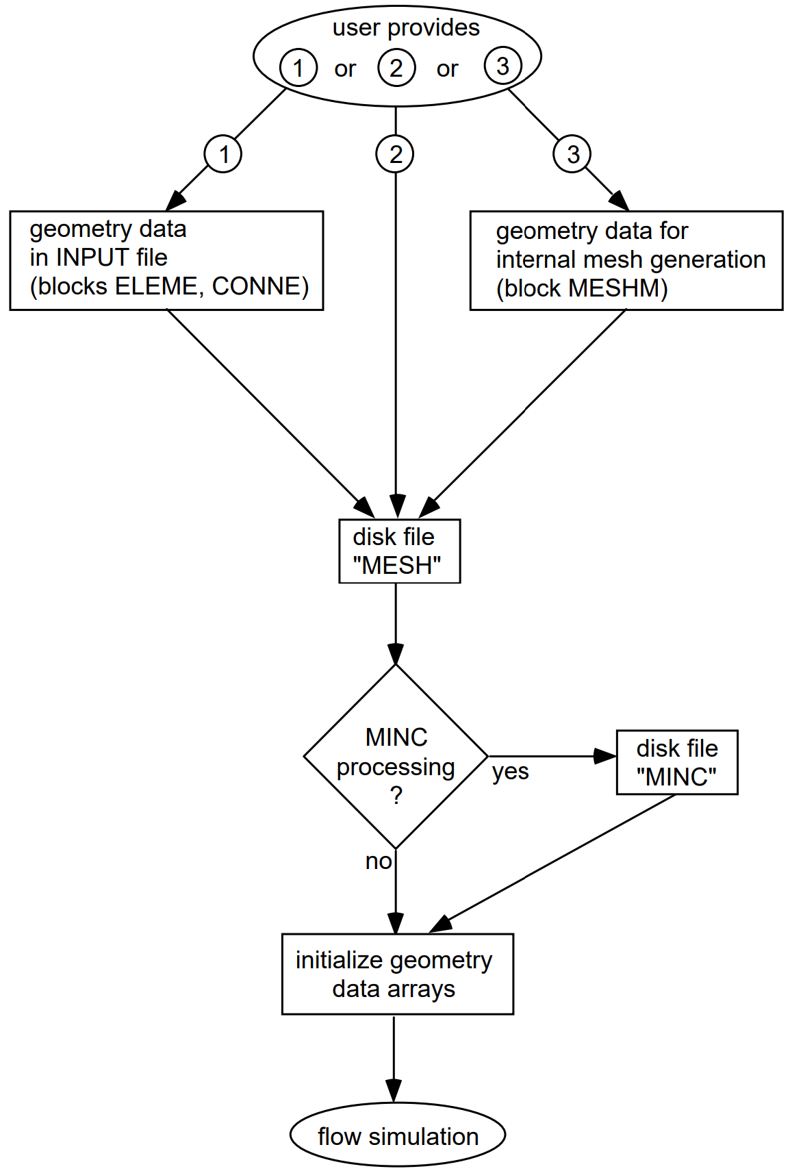
Figure 4 User options for supplying geometry data.

Meshmaker

TOUGH3 offers an additional way for defining flow system geometry by means of a special program module MESHMaker. This can perform a number of mesh generation and processing operations and is invoked with the keyword MESHM in the input file (see Figure 5). The MESHMaker module has a modular structure. At the present time, there are three sub-modules available in MESHMaker: keywords RZ2D or RZ2DL invoke generation of a one or two-dimensional radially symmetric R-Z mesh; XYZ initiates generation of a one, two, or three dimensional Cartesian X-Y-Z mesh; and MINC calls a modified version of the GMINC program (Pruess, 1983) to sub-partition a primary porous medium mesh into a secondary mesh for fractured media, using the method of “multiple interacting continua” (Pruess & Narasimhan, 1985), which will be described in detail below.

Several naming conventions for the elements created with keywords RZ2D (or RZ2DL) and XYZ have been adopted in the internal mesh generation process. In addition to the traditional TOUGH2 conventions, the other conventions are adopted to accommodate large numbers of grid blocks in cases with MOP2(2) > 5 or MOP2(27) > 0. Both RZ2D and XYZ assign all grid blocks to domain #1 (first entry in block ROCKS); a user desiring changes in domain assignments must do so by hand, either through editing of the MESH file with a text editor, or by means of preprocessing with an appropriate utility program, or by appropriate source code changes in subroutines WRZ2D and GXYZ. TOUGH3 runs that involve RZ2D or XYZ mesh generation will produce a special printout, showing element names arranged in their actual geometric pattern.

The naming conventions for the MINC process are as follows. For a primary grid block with name 12345, the corresponding fracture subelement in the secondary mesh is named 12345 (character #1 replaced with a blank for easy recognition). The successive matrix continua are labeled by running character #1 through 2, …, 9, A, B, …, Z. The domain assignment is incremented by 1 for the fracture grid blocks, and by 2 for the matrix grid blocks. Thus, domain assignments in data block ROCKS should be provided in the following order: the first entry is the single (effective) porous medium, then follows the effective fracture continuum, and then the rock matrix. Users should be aware that the MINC process may lead to ambiguous element names when the inactive element device is used to keep a portion of the primary mesh as unprocessed porous medium. Also, the MINC process may generate duplicate element names. TOUGH3 will check the element names after reading disk file MESH, and abort the simulation if duplicate element names are found.

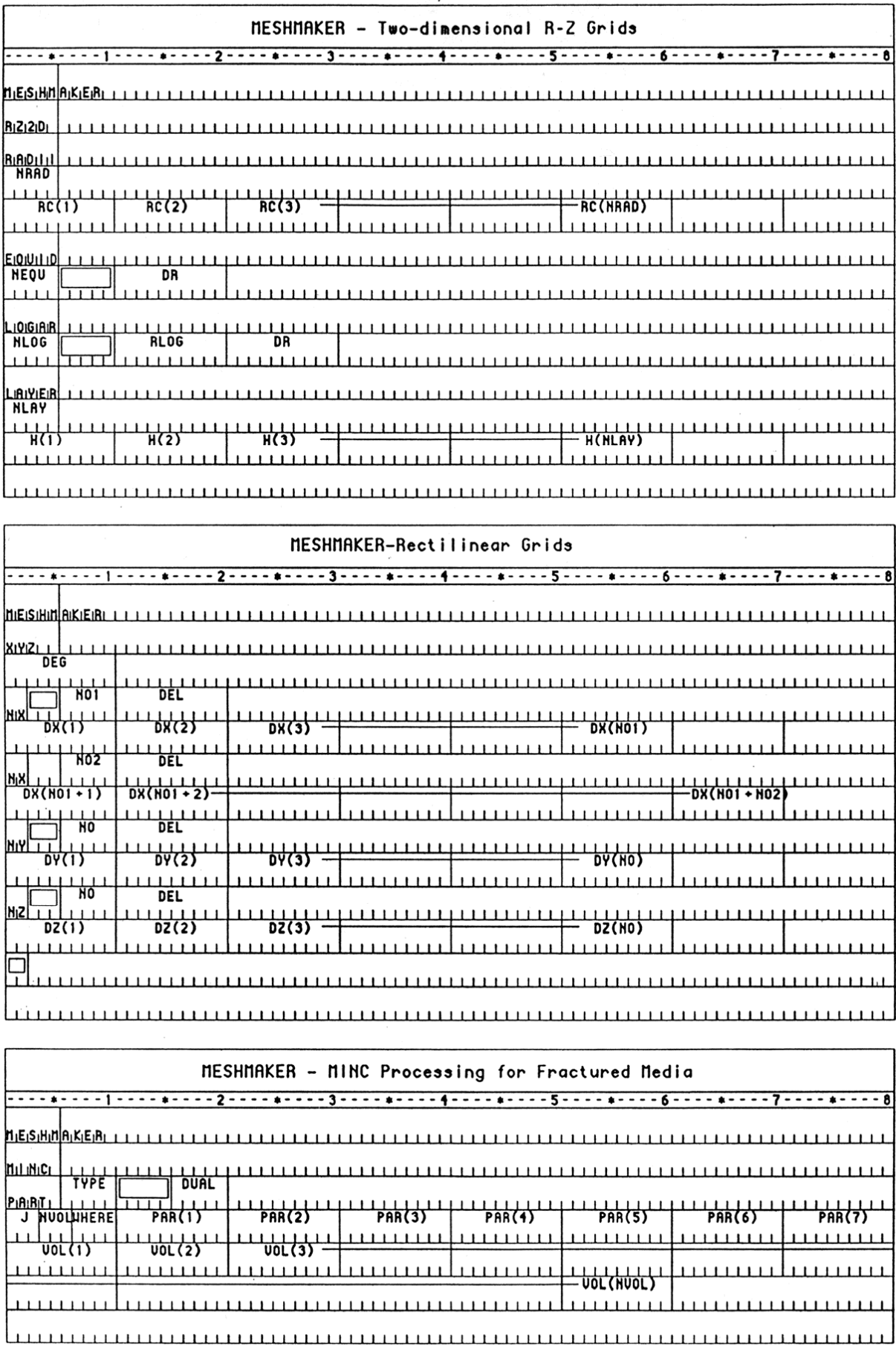
Figure 5 MESHMaker input formats.

As a convenience for users desiring graphical display of data, the internal mesh generation process will also write nodal point coordinates on file MESH. By default these data are written in 3E10.4 format into columns 51-80 of each grid block entry in data block ELEME, unless a longer effective digit of 3E20.14 format into columns 51-110 is specified in data block MOMOP (MOP2(22) > 0). No internal use is made of nodal point coordinates in TOUGH3, except for optional initialization of a gravity-capillary equilibrium with EOS9 (see the addendum for EOS9) and for optional addition of potential energy to enthalpy with MOP2(12) > 0 in data block MOMOP.

Mesh generation and/or MINC processing can be performed as part of a simulation run. Alternatively, by closing the input file with the keyword ENDFI (instead of ENDCY), it is possible to skip the flow simulation and only execute the MESHMaker module to generate a MESH or MINC file. These files can then be used, with additional user-modifications by hand if desired, in subsequent flow simulations. Execution of MESHMaker produces printed output which is self-explanatory.

Multiple-porosity processing

Multiple-porosity processing for simulation of flow in naturally fractured reservoirs can be invoked by means of a keyword MINC, which stands for “multiple interacting continua” (Pruess & Narasimhan, 1985). The MINC-process operates on the data of the primary (porous medium) mesh as provided on disk file MESH, and generates a “secondary” mesh containing fracture and matrix elements with identical data formats on file MINC. By appropriate subgridding of the matrix blocks, as shown in Figure 6, and therefore by resolving the driving pressure, temperature, and mass fraction gradients at the matrix and fracture interface, the transient, multiphase interporosity flows between rock matrix and fractures can accurately be described. The MINC concept is based on the notion that changes in fluid pressures, temperatures, phase compositions, etc, due to the presence of sinks and sources (production and injection wells) will propagate rapidly through the fracture system, while invading the tight matrix blocks only slowly. Therefore, changes in matrix conditions will (locally) be controlled by the distance from the fractures. Fluid and heat flow from the fractures into the matrix blocks, or from the matrix blocks into the fractures, can then be modeled by means of one-dimensional strings of nested grid blocks, as shown in Figure 6. The MINC-method lumps all fractions within a certain reservoir subdomain into continuum #1, all matrix material within a certain distance from the fractures into continuum #2, matrix material at larger distance into continuum #3, and so on. Quantitatively, the subgridding is specified by means of a set of volume fractions, into which the primary porous medium grid blocks are partitioned. The MINC-process in the MESHMaker module operates on the element and connection data of a porous medium mesh to calculate, for given data on volume fractions, the volumes, interface areas, and nodal distances for a secondary fractured medium mesh. The information on fracturing (spacing, number of sets, shape of matrix blocks) required for this is provided by a “proximity function” PROX(x) which expresses, for a given reservoir domain \(V_0\), the total fraction of matrix material within a distance \(x\) from the fractures. If only two continua are specified (one for fractures, one for matrix), the MINC approach reduces to the conventional double-porosity method (Warren & Root, 1963). Full details are given in a separate report (Pruess, 1983). For any given fractured reservoir flow problem, selection of the most appropriate gridding scheme must be based on a careful consideration of the physical and geometric conditions of flow. The MINC approach is not applicable to systems in which fracturing is so sparse that the fractures cannot be approximated as a continuum.

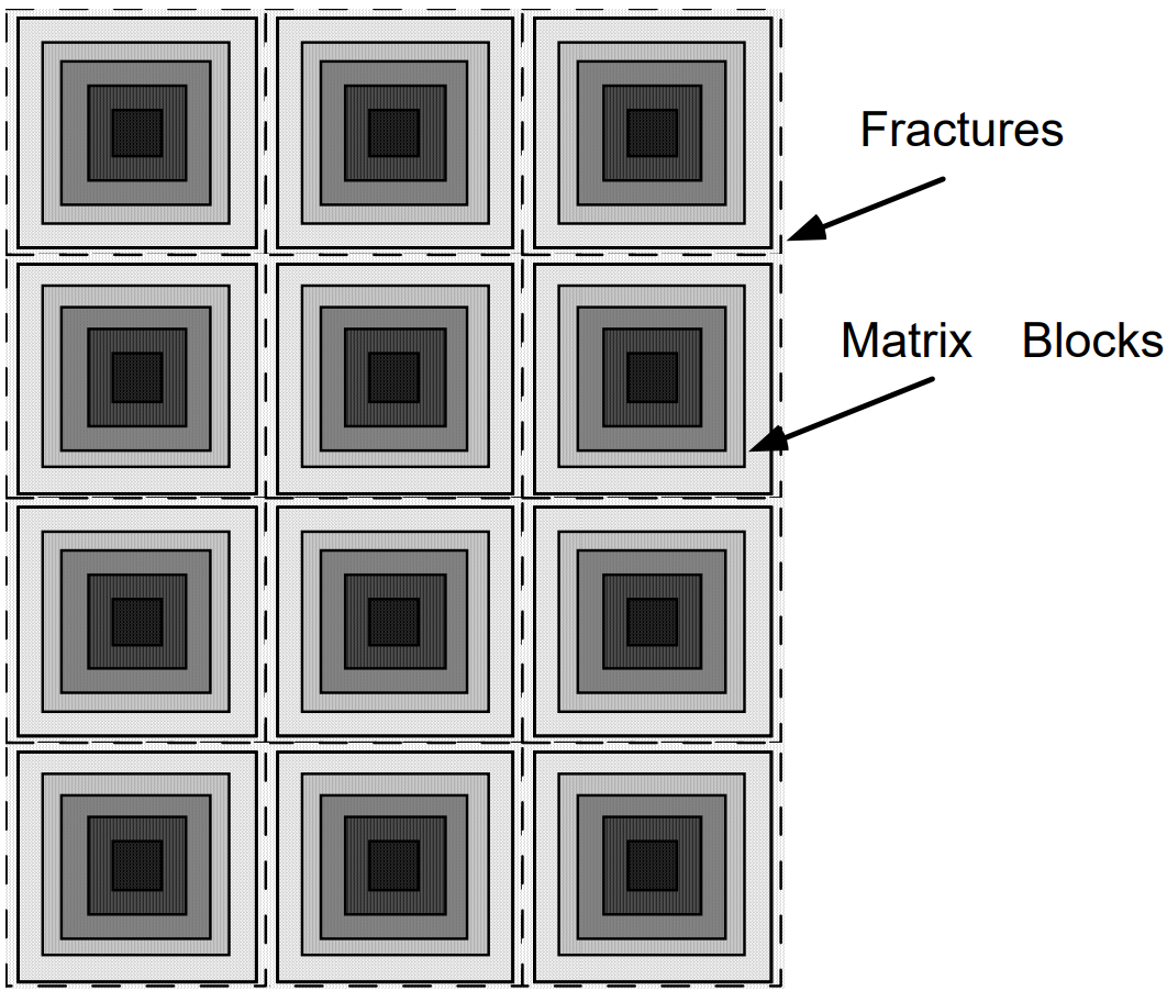
Figure 6 Subgridding in the method of “multiple interacting continua” (MINC).

The file MESH used in this process can be either directly supplied by the user, or it can have been internally generated either from data in input blocks ELEME and CONNE, or from RZ2D or XYZ mesh- making. The MINC process of sub-partitioning porous medium grid blocks into fracture and matrix continua will only operate on active grid blocks, while inactive grid blocks are left unchanged as single porous medium blocks. In TOUGH3, elements in data block ELEME (or file MESH) are taken to be “active” unless they have very large volumes, which are taken to be “inactive”. In order to exclude selected reservoir domains from the MINC process and make them remain single porous media, the user needs to change the volume of the corresponding blocks to a very large number before MINC partitioning is made. Note that here the concept of inactive blocks is used in an unrelated manner with respect to the one to maintain time-independent Dirichlet boundary conditions (see Section Initial and Boundary Conditions).

Input Formats for MESHMAKER

Generation of radially symmetric grid

Keyword RZ2D (or RZ2DL) invokes generation of a radially symmetric mesh. Nodal points will be placed half-way between neighboring radial interfaces. When RZ2D is specified, the mesh will be generated by columns; i.e., in the ELEME block we will first have the grid blocks at smallest radius for all layers, then the next largest radius for all layers, and so on. With keyword RZ2DL the mesh will be generated by layers; i.e., in the ELEME block we will first have all grid blocks for the first (top) layer from smallest to largest radius, then all grid blocks for the second layer, and so on. Apart from the different ordering of elements, the two meshes for RZ2D and RZ2DL are identical. The reason for providing the two alternatives is as a convenience to users in implementing boundary conditions by way of inactive elements (see Section Initial and Boundary Conditions). RZ2D makes it easy to declare a vertical column inactive, facilitating assignment of boundary conditions in the vertical, such as a gravitationally equilibrated pressure gradient. RZ2DL on the other hand facilitates implementation of areal (top and bottom layer) boundary conditions.

RADII

RADII is the first keyword following RZ2D; it introduces data for defining a set of interfaces (grid block boundaries) in the radial direction.

Table 51 Record RADII.1.

Parameter	Format	Description
NRAD	I5	number of radius data that will be read. At least one radius must be provided, indicating the inner boundary of the mesh.

Table 52 Record RADII.2.

Parameter	Format	Description
RC(I)	E10.4	I = 1, NRAD radii in ascending order.

EQUID

Introduces data on a set of equal radial increments.

Table 53 Record EQUID.1.

Parameter	Format	Description
NEQU	I5	number of desired radial increments.
	5X	(void)
DR	E10.4	number of desired radial increments.

Note that at least one radius must have been defined via block RADII before EQUID can be invoked.

LOGAR

Introduces data on radial increments that increase from one to the next by the same factor (\(\Delta R_{n + 1} = f \cdot \Delta R_n\)).

Table 54 Record LOGAR.1.

Parameter	Format	Description
NLOG	I5	number of additional interface radii desired.
	5X	(void)
RLOG	E10.4	desired radius of the last (largest) of these radii.
DR	E10.4	reference radial increment: the first \(\Delta R\) generated will be equal to f × DR, with f internally determined such that the last increment will bring total radius to RLOG. f < 1 for decreasing radial increments is permissible. If DR is set equal to zero, or left blank, the last increment DR generated before keyword LOGAR will be used as default.

Additional blocks RADII, EQUID, and LOGAR can be specified in arbitrary order. Note that at least one radius must have been defined before LOGAR can be invoked. If DR = 0, at least two radii must have been defined.

LAYER

Introduces information on horizontal layers, and signals closure of RZ2D input data.

Table 55 Record LAYER.1.

Parameter	Format	Description
NLAY	I5	number of horizontal grid layers.

Table 56 Record LAYER.2.

Parameter	Format	Description
H(I)	E10.4	I = 1, NLAY layer thicknesses, from top layer downward. By default, zero or blank entries for layer thickness will result in assignment of the last preceding non-zero entry. Assignment of a zero layer thickness, as needed for inactive layers, can be accomplished by specifying a negative value.

The LAYER data close the RZ2D data block. Note that one blank record must follow to indicate termination of the MESHM data block. Alternatively, keyword MINC can appear to invoke MINC-processing for fractured media (see below).

Generation of rectilinear grids

XYZ

Invokes generation of a Cartesian (rectilinear) mesh.

Table 57 Record XYZ.1.

Parameter	Format	Description
DEG	E10.4	angle (in degrees) between the Y-axis and the horizontal. If gravitational acceleration (parameter GF in record PARAM.2) is specified positive, -90° < DEG < 90° corresponds to grid layers going from top down. Grids can be specified from bottom layer up by setting GF or BETA negative. Default (DEG = 0) corresponds to horizontal Y- and vertical Z-axis. X-axis is always horizontal.

Table 58 Record XYZ.2.

Parameter	Format	Description
NTYPE	A2	set equal to NX, NY or NZ for specifying grid increments in X, Y, or Z direction.
	3X	(void)
NO	I5	number of grid increments desired.
DEL	E10.4	constant grid increment for NO grid blocks, if set to a non-zero value.

Table 59 Record XYZ.3.

Parameter	Format	Description
DEL(I)	E10.4	I = 1, NO grid increments in the direction specified by NTYPE in record XYZ.2. Additional records with formats as XYZ.2 and XYZ.3 can be provided, with X, Y, and Z-data in arbitrary order.

A blank record closes the XYZ data block.

Note that the end of block MESHMaker is also marked by a blank record. Thus, when MESHMaker/XYZ is used, there will be two blank records at the end of the corresponding input data block.

MINC processing for fractured media

MINC

Invokes postprocessing of a primary porous medium mesh from file MESH. The input formats in data block MINC are identical to those of the GMINC program (Pruess, 1983), with two enhancements: there is an additional facility for specifying global matrix-matrix connections (“dual permeability”); further, only active elements will be subjected to MINC-processing, the remainder of the MESH remaining unaltered as porous medium grid blocks.

PART

PART is the first keyword following MINC; it will be followed on the same line by parameters TYPE and DUAL with information on the nature of fracture distributions and matrix-matrix connections.

Table 60 Record PART.1.

Parameter	Format	Description
PART	A5	identifier of data block with partitioning parameters for secondary mesh.
TYPE	A5	a five-character word for selecting one of the six different proximity functions provided in MINC (Pruess, 1983): ONE-D: a set of plane parallel infinite fractures with matrix block thickness between neighboring fractures equal to PAR(1). TWO-D: two sets of plane parallel infinite fractures, with arbitrary angle between them. Matrix block thickness is PAR(1) for the first set, and PAR(2) for the second set. If PAR(2) is not specified explicitly, it will be set equal to PAR(1). THRED: three sets of plane parallel infinite fractures at right angles, with matrix block dimensions of PAR(1), PAR(2), and PAR(3), respectively. If PAR(2) and/or PAR(3) are not explicitly specified, they will be set equal to PAR(1) and/or PAR(2), respectively. STANA: average proximity function for rock loading of Stanford large reservoir model (Lam et al., 1988). STANB: proximity function for the five bottom layers of Stanford large reservoir model. STANT: proximity function for top layer of Stanford large reservoir model. Note: a user wishing to employ a different proximity function than provided in MINC needs to replace the function subprogram PROX(x) in file Mesh_Maker.f90 with a routine of the form: FUNCTION PROX(x) PROX = (arithmetic expression in x) RETURN END It is necessary that PROX(x) is defined even when x exceeds the maximum possible distance from the fractures, and that PROX = 1 in this case. Also, when the user supplies his/her own proximity function subprogram, the parameter TYPE has to be chosen equal to ONE-D, TWO-D, or THRED, depending on the dimensionality of the proximity function. This will assure proper definition of innermost nodal distance (Pruess, 1983).
	5X	(void)
DUAL	A5	a five-character word for selecting the treatment of global matrix matrix flow: blank: (default) global flow occurs only through the fracture continuum, while rock matrix and fractures interact locally by means of interporosity flow (“double-porosity” model). MMVER: global matrix-matrix flow is permitted only in the vertical; otherwise like the double-porosity model; for internal consistency this choice should only be made for flow systems with one or two predominantly vertical fracture sets. MMALL: global matrix-matrix flow in all directions; for internal consistency only two continua, representing matrix and fractures, should be specified (“dual-permeability”).

Table 61 Record PART.2.

Parameter	Format	Description
J	I3	total number of multiple interacting continua.
NVOL	I3	total number of explicitly provided volume fractions (NVOL < J). If NVOL < J, the volume fractions with indices NVOL + 1, …, J will be internally generated; all being equal and chosen such as to yield proper normalization to 1.
WHERE	A4	specifies whether the sequentially specified volume fractions begin with the fractures (WHERE = OUT) or in the interior of the matrix blocks (WHERE = IN).
PAR(I)	E10.4	I = 1, 7 holds parameters for fracture spacing (see above).

Table 62 Record PART.2.1.

Parameter	Format	Description
VOL(I)	E10.4	I = 1, NVOL volume fraction (between 0 and 1) of continuum with index I (for WHERE = OUT) or index J + 1 - I (for WHERE = IN). NVOL volume fractions will be read. For WHERE = OUT , I = 1 is the fracture continuum, I = 2 is the matrix continuum closest to the fractures, I = 3 is the matrix continuum adjacent to I = 2, etc. The sum of all volume fractions must not exceed 1.