Numerical Methods

Space and Time Discretization

TOUGH3 uses an integral finite difference method for space discretization, and first-order fully implicit time differencing. The resulting strongly coupled, nonlinear algebraic equations are solved simultaneously using Newton-Raphson iterations for each time step, which involves the calculation of a Jacobian matrix and the solution of a set of linear equations. Time steps are automatically adjusted during a simulation run, depending on the convergence rate of the iteration process. Newton-Raphson increment weighting can also be adjusted if the iterations oscillate.

The continuum equations Eq. (1) are discretized in space using the integral finite difference method (IFD; Narasimhan & Witherspoon, 1976). Introducing appropriate volume averages, we have

(31)\[\int_{V_n} M dV = V_n M_n\]

where \(M\) is a volume-normalized extensive quantity, and \(M_n\) is the average value of \(M\) over \(V_n\).

Surface integrals are approximated as a discrete sum of averages over surface segments \(A_{nm}\):

(32)\[\int_{\Gamma_n} \boldsymbol{\mathrm{F}}^{\kappa} \cdot \boldsymbol{\mathrm{n}} d\Gamma_n = \sum_{m} A_{nm} F_{nm}\]

Here, \(F_{nm}\) is the average value of the (inward) normal component of \(\boldsymbol{\mathrm{F}}\) over the surface segment \(A_{nm}\) between volume elements \(V_n\) and \(V_m\). The discretization approach used in the integral finite difference method and the definition of the geometric parameters are illustrated in Figure 2.

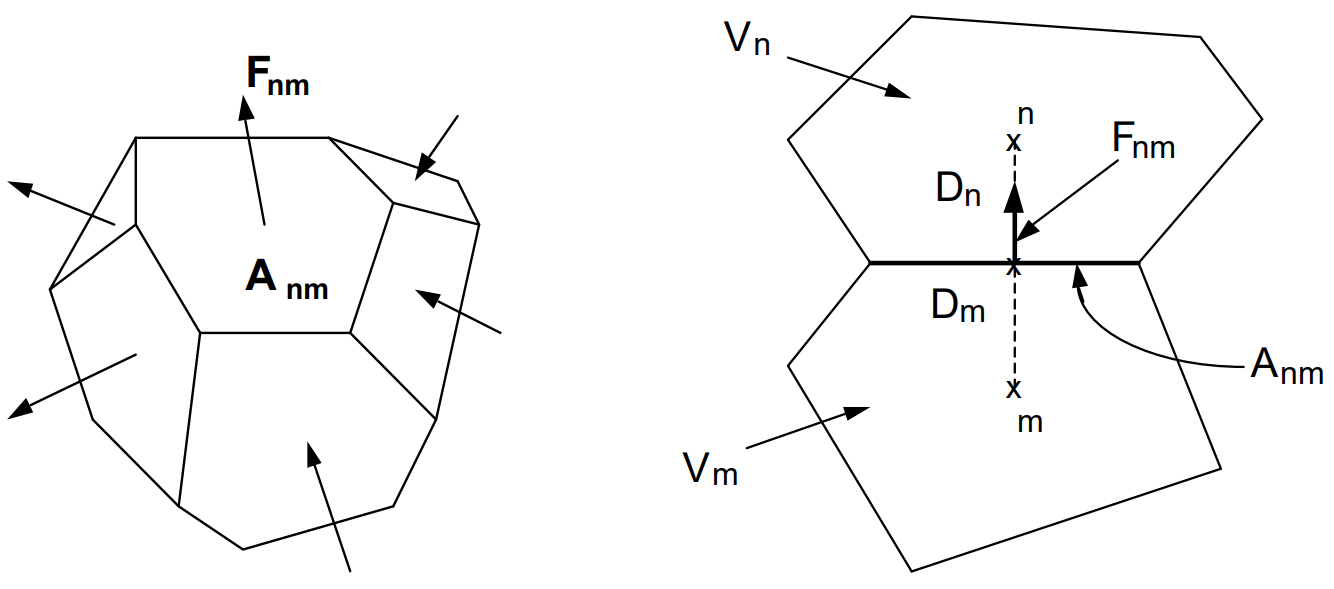
Figure 2 Space discretization and geometry data in the integral finite difference method.

The discretized flux is expressed in terms of averages over parameters for elements \(V_n\) and \(V_m\). For the basic Darcy flux term, Eq. (5), we have

(33)\[F_{\beta, nm} = -k_{nm} \left( \frac{k_{r \beta} \rho_{\beta}}{\mu_{\beta}} \right)_{nm} \left( \frac{P_{\beta, n} - P_{\beta, m}}{D_{nm}} \rho_{\beta, nm} g_{nm} \right)\]

where the subscripts \((nm)\) denote a suitable averaging at the interface between grid blocks \(n\) and \(m\) (such as interpolation, harmonic weighting, and upstream weighting, which will be discussed in Section Interface Weighting Schemes). \(D_{nm} = D_n + D_m\) is the distance between the nodal points \(n\) and \(m\), and \(g_{nm}\) is the component of gravitational acceleration in the direction from \(m\) to \(n\).

Space discretization of diffusive flux in multiphase conditions raises some subtle issues. A finite difference formulation for total diffusive flux, Eq. (11), may be written as

(34)\[\left( f^{\kappa} \right)_{nm} = - \left( \Sigma_l^{\kappa} \right)_{nm} \frac{\left( X_l^{\kappa} \right)_m - \left( X_l^{\kappa} \right)_n}{D_{nm}} - \left( \Sigma_g^{\kappa} \right)_{nm} \frac{\left( X_g^{\kappa} \right)_m - \left( X_g^{\kappa} \right)_n}{D_{nm}}\]

This expression involves the as yet unknown diffusive strength coefficients \(\left( \Sigma_l^{\kappa} \right)_{nm}\) and \(\left( \Sigma_g^{\kappa} \right)_{nm}\) at the interface, which must be expressed in terms of the strength coefficients in the participating grid blocks. Invoking conservation of diffusive flux across the interface between two grid blocks leads in the usual way to the requirement of harmonic weighting of the diffusive strength coefficients. However, such weighting may in general not be applied separately to the diffusive fluxes in gas and liquid phases, because these may be strongly coupled by phase partitioning effects. This can be seen by considering the extreme case of diffusion of a water-soluble and volatile compound from a grid block in single-phase gas conditions to an adjacent grid block which is in single-phase liquid conditions. Harmonic weighting applied separately to liquid and gas diffusive fluxes would result in either of them being zero, because for each phase effective diffusivity is zero on one side of the interface. Thus total diffusive flux would vanish in this case, which is unphysical. In reality, tracer would diffuse through the gas phase to the gas-liquid interface, would establish a certain mass fraction in the aqueous phase by dissolution, and would then proceed to diffuse away from the interface through the aqueous phase. Similar arguments can be made in the less extreme situation where liquid saturation changes from a large to a small value rather than from 1 to 0, as may be the case in the capillary fringe, during infiltration events, or at fracture-matrix interfaces in variably saturated media.

TOUGH3 features a fully coupled approach in which the space-discretized version Eq. (34) of the total multiphase diffusive flux Eq. (11) is re-written in terms of an effective multiphase diffusive strength coefficient and a single mass fraction gradient. Choosing the liquid mass fraction for this we have

(35)\[\left( f^{\kappa} \right)_{nm} = - \left\{ \Sigma_l^{\kappa} + \Sigma_g^{\kappa} \frac{\left( X_g^{\kappa} \right)_m - \left( X_g^{\kappa} \right)_n}{\left( X_l^{\kappa} \right)_m - \left( X_l^{\kappa} \right)_n} \right\}_{nm} \frac{\left( X_l^{\kappa} \right)_m - \left( X_l^{\kappa} \right)_n}{D_{nm}}\]

where the gas phase mass fraction gradient has been absorbed into the effective diffusive strength term (in braces). As is well known, flux conservation at the interface then leads to the requirement of harmonic weighting for the full effective strength coefficient. In order to be able to apply this scheme to the general case where not both phases may be present on both sides of the interface, we always define both liquid and gas phase mass fractions in all grid blocks, regardless of whether both phases are present. Mass fractions are assigned in such a way as to be consistent with what would be present in an evolving second phase. This procedure is applicable to all possible phase combinations, including the extreme case where conditions at the interface change from single-phase gas to single-phase liquid. Note that, if the diffusing tracer exists in just one of the two phases, harmonic weighting of the strength coefficient in Eq. (35) will reduce to harmonic weighting of either \(\Sigma_l^{\kappa}\) or \(\Sigma_g^{\kappa}\). The simpler scheme of separate harmonic weighting for individual phase diffusive fluxes is retained as an option.

Substituting Eqs. (31) and (32) into the governing Eq. (1), a set of first-order ordinary differential equations in time is obtained:

(36)\[\frac{dM_n^{\kappa}}{dt} = \frac{1}{V_n} \sum_m A_{nm} F_{nm}^{\kappa} + q_n^{\kappa}\]

Time is discretized as a first-order finite difference, and the flux and sink and source terms on the right-hand side of Eq. (36) are evaluated at the new time level, \(t^{k + l} = t^k + \Delta t\), to obtain the numerical stability needed for an efficient calculation of multiphase flow. This treatment of flux terms is known as “fully implicit”, because the fluxes are expressed in terms of the unknown thermodynamic parameters at time level \(k + 1\), so that these unknowns are only implicitly defined in the resulting equations (see, e.g., Peaceman, 2000). The time discretization results in the following set of coupled nonlinear, algebraic equations

(37)\[R_n^{\kappa, k+1} = M_n^{\kappa, k+1} - R_n^{\kappa, k} \frac{\Delta t}{V_n} \left( \sum_m A_{nm} F_{nm}^{\kappa, k+1} + V_n q_n^{\kappa, k+1} \right) = 0\]

where we have introduced residuals \(R_n^{\kappa, k+1}\). For each volume element (grid block) \(V_n\), there are \(NEQ\) mass and heat balance equations (\(\kappa = 1, 2, ..., NEQ\), where \(NEQ\) represents the number of equations per grid block). For a flow system with \(NEL\) grid blocks, Eq. (37) represents a total of \(NEL \times NEQ\) coupled nonlinear equations. The unknowns are the \(NEL \times NEQ\) independent primary variables \(\left\{ x_i; i = 1, ..., NEL \times NEQ \right\}\) which completely define the state of the flow system at time \(t^{k + l}\). These equations are solved by Newton-Raphson iteration, which is implemented as follows. We introduce an iteration index \(p\) and expand the residuals \(R_n^{\kappa, k+1}\) in Eq. (37) at iteration step \(p + 1\) in a Taylor series in terms of the residuals at index \(p\).

(38)\[R_n^{\kappa, k+1} \left( x_{i, p+1} \right) = R_n^{\kappa, k+1} \left( x_{i, p} \right) + \sum_i \frac{\partial R_n^{\kappa, k+1}}{\partial x_i} \bigg|_p \left( x_{i, p+1} - x_{i, p} \right) + ... = 0\]

Retaining only terms up to first order, we obtain a set of \(NEL \times NEQ\) linear equations for the increments \(\left( x_{i, p+1} - x_{i, p} \right)\):

(39)\[- \sum_i \frac{\partial R_n^{\kappa, k+1}}{\partial x_i} \bigg|_p \left( x_{i, p+1} - x_{i, p} \right) = R_n^{\kappa, k+1} \left( x_{i, p} \right)\]

All terms \(\partial R_n / \partial x_i\) in the Jacobian matrix are evaluated by numerical differentiation. Eq. (39) is solved by the linear equations solver selected. Iteration is continued until the residuals \(R_n^{\kappa, k+1}\) are reduced below a preset convergence tolerance.

(40)\[\left\vert \frac{R_{n, p+1}^{\kappa, k+1}}{M_{n, p+1}^{\kappa, k+1}} \right\vert \le \varepsilon_1\]

The default (relative) convergence criterion is \(\varepsilon_1 = 10^{-5}\). When the accumulation terms are smaller than \(\varepsilon_2\) (default \(\varepsilon_2 = 1\)), an absolute convergence criterion is imposed.

(41)\[\left\vert R_n^{\kappa, k+1} \right\vert \le \varepsilon_1 \cdot \varepsilon_2\]

Convergence is usually attained in 3 to 4 iterations. If convergence cannot be achieved within a certain number of iterations (default 8), the time step size \(\Delta t\) is reduced and a new iteration process is started.

It is appropriate to add some comments about this space discretization technique. The entire geometric information of the space discretization in Eq. (37) is provided in the form of a list of grid block volumes \(V_n\), interface areas \(A_{nm}\), nodal distances \(D_{nm}\) and components \(g_{nm}\) of gravitational acceleration along nodal lines. There is no reference whatsoever to a global system of coordinates, or to the dimensionality of a particular flow problem. The discretized equations are in fact valid for arbitrary irregular discretizations in one, two or three dimensions, and for porous as well as for fractured media. This flexibility should be used with caution, however, because the accuracy of solutions depends upon the accuracy with which the various interface parameters in equations such as Eq. (33) can be expressed in terms of average conditions in grid blocks. A general requirement is that there exists approximate thermodynamic equilibrium in (almost) all grid blocks at (almost) all times (Pruess & Narasimhan, 1985). For systems of regular grid blocks referenced to global coordinates (such as \(r-z\) or \(x-y-z\)), Eq. (37) is identical to a conventional finite difference formulation (e.g., Moridis, 1992, Peaceman, 2000).

Interface Weighting Schemes

To obtain a reasonably accurate and efficient solution, particularly for multiphase fluid and heat flow problems, a proper interface weighting scheme should be used. It is well known that for single-phase flow, the appropriate interface weighting scheme for absolute permeability is harmonic weighting. For two-phase flow, the added problem of relative permeability weighting arises. It has been established that for transient flow problems in homogeneous media, relative permeability must be upstream weighted, or else phase fronts may be propagated with erroneous speed (Aziz & Settari, 1979). Studies at the Lawrence Berkeley National Laboratory have shown that for transient two-phase problems in composite (layered) media, both absolute and relative permeability must be fully upstream weighted to avoid the possibility of gross errors (Tsang & Pruess, 1990, Wu et al., 1993). The applicable weighting schemes for different flow problems are summarized in Figure 3. There is no single weighting scheme for general two-phase flows in composite media that would at the same time preserve optimal accuracy for single-phase or steady two-phase flows.

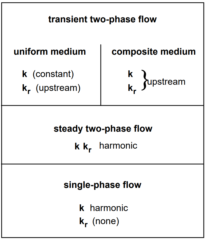
Figure 3 Weighting procedures for absolute (\(k\)) and relative permeability (\(k_r\)) at grid block interfaces.

For modeling of fracture-matrix interaction, a different weighting scheme can be applied. If a zero nodal distance is specified, the absolute (and relative, if MOP2(7) > 0) permeability from the other element is used for assignment of interface mobilities.

Another interesting problem is the weighting scheme for interface densities. For proper modeling of gravity effects, it is necessary to define interface density as the arithmetic average between the densities of the two adjacent grid blocks, regardless of nodal distances from the interface. An unstable situation may arise when phases (dis-)appear, because interface density may then have to be “switched” to the upstream value when the phase in question is not present in the downstream block. For certain flow problems, spatial interpolation of densities may provide more accurate answers.

Issues of interface weighting and associated discretization errors are especially important when non-uniform or irregular grids are used. Additional complications related to interface weighting arise in flow problems that involve hydrodynamic instabilities. Examples include immiscible displacements with unfavorable mobility ratio where a less viscous fluid displaces a fluid of higher viscosity (viscous instability), and flow problems where a denser fluid invades a zone with less dense fluid from above (gravity instability). These instabilities can produce very large grid orientation errors, i.e., simulated results can depend strongly on the orientation of the computational grid (Pruess, 1991, Pruess & Bodvarsson, 1983, Yanosik & McCracken, 1979).

In some cases, it may be advisable to use higher-order differencing schemes. Grid orientation effects can be reduced by using 7-point or 9-point differencing instead of the common 5-point “stencil”, to achieve a higher degree of rotational invariance in the finite difference approximations of the fundamental differential operators. In the integral finite difference method, these higher-order schemes can be implemented through preprocessing of geometry data, without any coding changes, by assigning additional flow connections with appropriate weighting factors between elements of the computational grid (Pruess, 1991, Pruess & Bodvarsson, 1983). However, reduction or elimination of grid orientation effects as such does not necessarily achieve a better numerical approximation. It may just amount to reducing the anisotropy of space discretization errors but not their magnitude, creating an illusion of a better approximation by making space discretization effects less obvious (Pruess, 1991).

Linear Equation Solvers

TOUGH3 offers a choice of linear solvers: the internal serial linear solvers of TOUGH2, the parallel Aztec solvers (Tuminaro et al., 1999; used in TOUGH2-MP), and all the serial and parallel solvers available in Portable, Extensible Toolkit for Scientific Computation (PETSc) (Balay et al., 2016). TOUGH3 provides a common interface to all three sources of linear solvers, allowing users to experiment with different solvers and their preconditioners, and to determine the most efficient method for the problem of interest. In addition, there is no restriction on using the Aztec and PETSc solvers in serial mode. Moreover, the internal serial solvers included in TOUGH3 are updated with a new sorting algorithm (private communication, Navarro, 2015), which results in a performance gain up to 30% when compared with the serial solvers in TOUGH2 (actual performance gains are problem-specific). The different linear equation solvers included in the TOUGH3 package can be selected by means of parameter MOP(21) in data block PARAM.1 (see Section 8.2).

Internal serial solvers

The most reliable linear equation solvers are based on direct methods, while the performance of iterative techniques tends to be problem-specific and lacks the predictability of direct solvers. The robustness of direct solvers comes at the expense of large storage requirements and execution times that typically increase proportional to \(N^3\), where \(N\) is the number of equations to be solved. In contrast, iterative solvers have much lower memory requirements, and their computational work increases much less rapidly with problem size, approximately proportional to \(N^{\omega}\), with \(\omega \approx 1.4 - 1.6\) (Moridis & Pruess, 1995). For large problems (especially 3D problems with more than several thousand volume elements), iterative conjugate gradient (CG) type solvers are therefore the method of choice. Technical details of the serial methods and their performance can be found in Moridis & Pruess, 1998.

TOUGH3 includes several internal serial solvers: one direct solver, LUBAND, and four iterative solvers, DSLUBC (bi-conjugate gradient solver), DSLUCS (Lanczos-type bi-conjugate gradient solver), DSLUGM (generalized minimum residual solver), and DLUSTB (stabilized bi-conjugate gradient solver). By default, TOUGH3 uses DSLUCS with incomplete LU-factorization as preconditioner for serial runs. Users need to beware that iterative methods may fail for matrices with special features, such as many zeros on the main diagonal, large numerical range of matrix elements, and nearly linearly dependent rows or columns. Depending on features of the problem at hand, appropriate matrix preconditioning may be essential to achieve convergence. Poor accuracy of the linear equation solution will lead to deteriorated convergence rates for the Newton-Raphson iteration, and an increase in the number of iterations for a given time step. In severe cases, time steps may fail with residuals either stagnating or wildly fluctuating. Users experiencing difficulties with the default settings are encouraged to experiment with the various solvers and preconditioners included in the TOUGH3 package.

All iterative solvers use incomplete LU-factorization as a preconditioner. Alternative preconditioners and iteration parameters can be selected by means of an optional data block SOLVR in the TOUGH3 input file. If SOLVR is present, its specifications will override the choices made by MOP(21). The default preconditioning with SOLVR is also incomplete LU-factorization.

The solver DLUSTB implements the BiCGSTAB(m) algorithm (Sleijpen & Fokkema, 1993), an extension of the BiCGSTAB algorithm of Vorst, 1992. DLUSTB provides improved convergence behavior when iterations are started close to the solution, i.e., near steady state. The preconditoning algorithms (the Z-preprocessors) can cope with difficult problems in which many of the Jacobian matrix elements on the main diagonal are zero. An example is the “two-waters” problem with EOS1 in which typically 2/3 of the elements in the main diagonal are zero. Moridis & Pruess, 1998 show that this type of problem can be solved by choosing appropriate pre-processing options.

PETSc solvers

TOUGH3 provides access to PETSc-based sparse and dense linear solvers. In many cases, the PETSc solvers are more efficient than the original serial solvers and the Aztec solvers. Since PETSc is being continually updated, users should consult PETSc’s documentation (http://www.mcs.anl.gov/petsc/documentation/index.html) and the summary of the linear solvers available from PETSc (http://www.mcs.anl.gov/petsc/documentation/linearsolvertable.html) for a list of updated Krylov subspace algorithms and preconditioners [5].

The current default PETSc solver is the bi-conjugate gradient method with incomplete LU factorization as the preconditioner. Different Krylov subspace algorithms and preconditioners can be selected through the specification of a PETSc option file (.petscrc), an example of which is shown below:

Listing 1 An example of the PETSc option file (.petscrc).

# monitor solves
-ksp_monitor
# biconjugate gradient
-ksp_type bicg
# additive Schwarz preconditioner
-pc_type asm
# relative tolerance
-ksp_rtol 1e-7

Commonly used options are shown in Table Table 1.

Table 1 Commonly used options for PETSc linear solvers.

Keywords	Description	Options
ksp_type	Solvers	bigcg (bi-conjugate gradient method) bcgsl (stabilized version of bi-conjugate gradient method) cg (conjugate gradient method) minres (minimum residual gradient) gmres (generalized minimal residual method) fgmres (flexible generalized minimal residual method)
pc_type	preconditioner	jacobi (point Jacobi preconditioner) pcjacobi (point block Jacobi preconditioner) bjacobi (block Jacobi preconditioner) asm (restricted additive Schwarz method) ilu (incomplete factorization preconditioner) icc (incomplete Cholesky factorization preconditioner) jacobi (diagonal scaling preconditioning)
ksp_monitor	monitor convergence	N/A. Refer to http://www.mcs.anl.gov/petsc/petsc-current/docs/manualpages/KSP/KSPMonitorSet.html for alternatives.
ksp_rtol	relative convergence tolerance	Any real number.

We do not provide the ability to set these options through the SOLVR block since it is difficult to encode the various options into the structure of the SOLVR block. In addition, the use of a separate option file ensures easy access to PETSc’s latest linear solvers and its diagnostic tools.

A special case is when using dense linear solver. Then, the user will set ksp_type to none and pc_type to lu. Note that LU decomposition only works in serial mode. To use dense linear solvers in parallel, changes can be made to the PETSc configuration scripts to include the parallel dense linear solver MUMPS and SuperLU.

[5]

In TOUGH3, the PETSc libraries are configured without any external linear solver packages such as MUMPS and SuperLU. However, these packages can be easily included through minor changes to the configuration script.

Aztec solvers

TOUGH3 provides an interface to Aztec solvers, but users should note that the version of the Aztec solver in TOUGH3 is no longer actively maintained. The PETSc solvers are in general more efficient than the Aztec solvers, but the Aztec solvers can be more efficient when the number of variables per core is small.

Consistent with the implementation of the PETSc solvers, the options available in Aztec can be set through the specification of an Aztec option file (.aztecrc). An example is shown below:

Listing 2 An example of the Aztec option file (.aztecrc).

AZ_solver AZ_bicgstab
AZ_precond AZ_dom_decomp
AZ_tol 1e-6

The format of the Aztec option file is inherited from TOUGH2-MP. TOUGH3 allows the user to modify nearly all Aztec options and parameters described in Section 2 of the Aztec manual (http://www.cs.sandia.gov/CRF/pspapers/Aztec_ug_2.1.ps) through .aztecrc. User can also refer to the TOUGH2-MP manual for more details.