ECO2N

Injection of CO₂ into saline formations has been proposed as a means whereby emissions of heat-trapping greenhouse gases into the atmosphere may be reduced. Such injection would induce coupled processes of multiphase fluid flow, heat transfer, chemical reactions, and mechanical deformation. Several groups have developed simulation models for subsets of these processes. The present report describes a fluid property module “ECO2N” for the general-purpose reservoir simulator TOUGH2 (Pruess, 2004, Pruess et al., 1999), that can be used to model non-isothermal multiphase flow in the system H₂O - NaCl - CO₂. TOUGH2/ECO2N represents fluids as consisting of two phases: a water-rich aqueous phase, herein often referred to as “liquid”, and a CO₂-rich phase referred to as “gas”. In addition, solid salt may also be present. The only chemical reactions modeled by ECO2N include equilibrium phase partitioning of water and carbon dioxide between the liquid and gaseous phases, and precipitation and dissolution of solid salt. The partitioning of H₂O and CO₂ between liquid and gas phases is modeled as a function of temperature, pressure, and salinity, using the recently developed correlations of Spycher et al., 2003. Dissolution and precipitation of salt is treated by means of local equilibrium solubility. Associated changes in fluid porosity and permeability may also be modeled. All phases - gas, liquid, solid - may appear or disappear in any grid block during the course of a simulation. Thermodynamic conditions covered include a temperature range from ambient to 100˚C (approximately), pressures up to 600 bar, and salinity from zero to fully saturated. These parameter ranges should be adequate for most conditions encountered during disposal of CO₂ into deep saline aquifers.

Theoretical Background

Fluid Phases and Thermodynamic Variables in the System Water-NaCl-CO₂

In the two-component system water-CO₂, at temperatures above the freezing point of water and not considering hydrate phases, three different fluid phases may be present: an aqueous phase that is mostly water but may contain some dissolved CO₂, a liquid CO₂-rich phase that may contain some water, and a gaseous CO₂-rich phase that also may contain some water. Altogether there may be seven different phase combinations (Figure 10). If NaCl (“salt”) is added as a third fluid component, the number of possible phase combinations doubles, as in each of the seven phase combinations depicted in Figure 10 there may or may not be an additional phase consisting of solid salt. Liquid and gaseous CO₂ may coexist along the saturated vapor pressure curve of CO₂, which ends at the critical point (\(T_{crit}\), \(P_{crit}\)) = (31.04˚C, 73.82 bar; Vargaftik, 1975), see Figure 11. At supercritical temperatures or pressures there is just a single CO₂-rich phase.

Figure 10 Possible phase combinations in the system water-CO₂. The phase designations are a - aqueous, l - liquid CO₂, g - gaseous CO₂. Separate liquid and gas phases exist only at subcritical conditions.

The present version of ECO2N can only represent a limited subset of the phase conditions depicted in Figure 10. Thermophysical properties are accurately calculated for gaseous as well as for liquid CO₂, but no distinction between gaseous and liquid CO₂ phases is made in the treatment of flow, and no phase change between liquid and gaseous CO₂ is treated. Accordingly, of the seven phase combinations shown in Figure 10, ECO2N can represent the ones numbered 1 (single-phase aqueous with or without dissolved CO₂ and salt), 2 and 3 (a single CO₂-rich phase that may be either liquid or gaseous CO₂, and may include dissolved water), and 4 and 5 (two-phase conditions consisting of an aqueous and a single CO₂-rich phase, with no distinction being made as to whether the CO₂-rich phase is liquid or gas). ECO2N cannot represent conditions 6 (two-phase mixture of liquid and gaseous CO₂) and 7 (three-phase). All sub- and super-critical CO₂ is considered as a single non-wetting phase, that will henceforth be referred to as “gas”. ECO2N may be applied to sub- as well as super-critical temperature and pressure conditions, but applications that involve sub-critical conditions are limited to systems in which there is no change of phase between liquid and gaseous CO₂, and in which no mixtures of liquid and gaseous CO₂ occur.

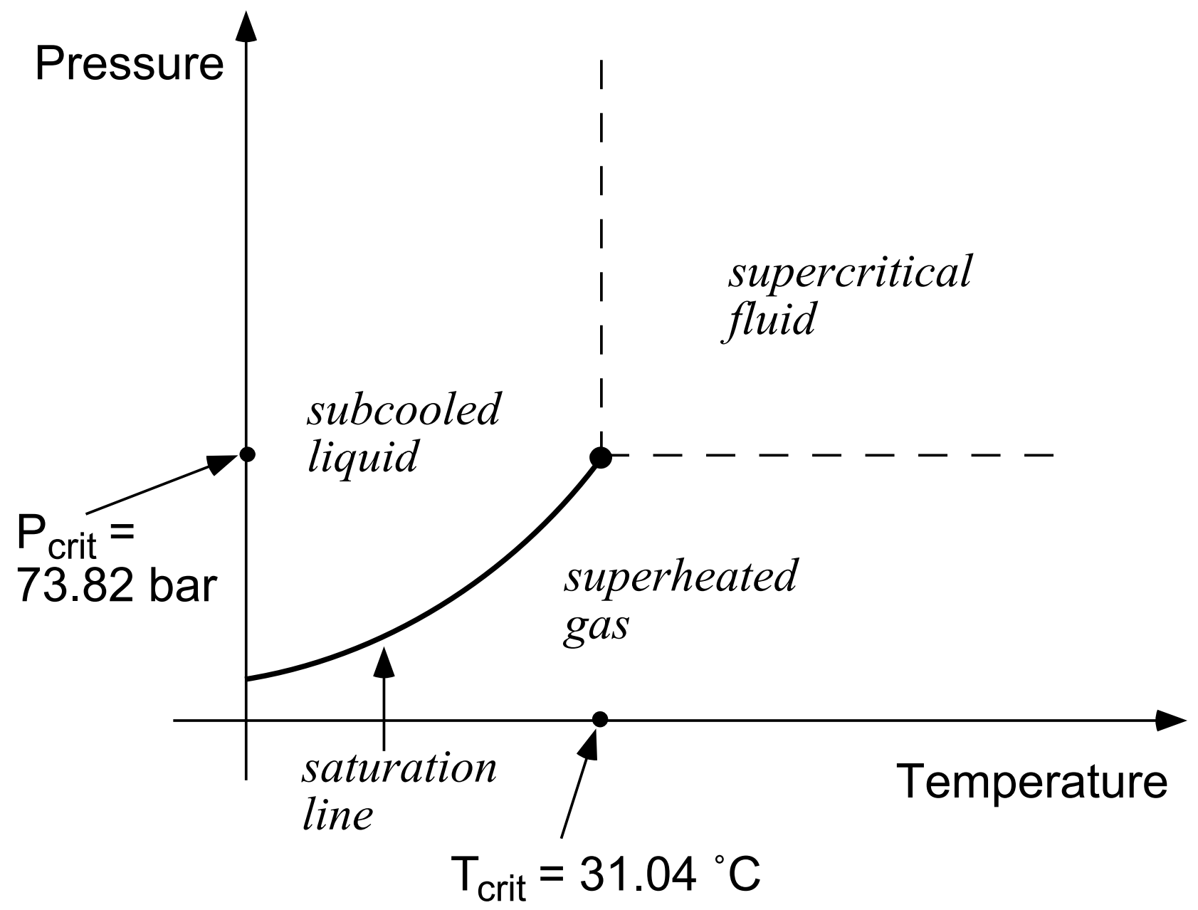
Figure 11 Phase states of CO₂.

Numerical modeling of the flow of brine and CO₂ requires a coupling of the phase behavior of water-salt-CO₂ mixtures with multiphase flow simulation techniques. Among the various issues raised by such coupling is the choice of notation. There are long-established notational conventions in both fields, which may lead to conflicts and misunderstandings when they are combined. In an effort to avoid confusion, we will briefly discuss notational issues pertaining to partitioning of CO₂ between an aqueous and a gaseous phase.

Phase partitioning is usually described in terms of mole fractions of the two components, which are denoted by \(x\) and \(y\), respectively, where \(x_1\) = \(x_{H_2O}\) and \(x_2\) = \(x_{CO_2}\) specify mole fractions in the aqueous phase, while \(y_1\) = \(y_{H_2O}\) and \(y_2\) = \(y_{CO_2}\) give mole fractions in the gas phase (Prausnitz et al., 1998, Spycher et al., 2003). We follow this notation, except that we add the subscript “eq” to emphasize that these mole fractions pertain to equilibrium partitioning of water and CO₂ between co-existing aqueous and gas phases. Accordingly, we denote the various mole fractions pertaining to equilibrium phase partitioning as \(x_{1, eq}\), \(x_{2, eq}\), \(y_{1, eq}\), and \(y_{2, eq}\), while the corresponding mass fractions are denoted using upper-case X and Y. Mass fractions corresponding to single-phase conditions, where water and CO₂ concentrations are not constrained by phase equilibrium relations, are denoted by \(X_1\) (for water) and \(X_2\) (for CO₂) in the aqueous phase, and by \(Y_1\) and \(Y_2\) in the gas phase.

In the numerical simulation of brine-CO₂ flows, we will be concerned with the fundamental thermodynamic variables that characterize the brine-CO₂ system, and their change with time in different subdomains (grid blocks) of the flow system. Four “primary variables” are required to define the state of water-NaCl-CO₂ mixtures, which according to conventional TOUGH2 useage are denoted by \(X_1\), \(X_2\), \(X_3\), and \(X_4\). A summary of the fluid components and phases modeled by ECO2N, and the choice of primary thermodynamic variables, appears in Table 100. Different variables are used for different phase conditions, but two of the four primary variables are the same, regardless of the number and nature of phases present. This includes the first primary variable \(X_1\), denoting pressure, and the fourth primary variable \(X_4\) which is temperature. The second primary variable pertains to salt and is denoted \(X_{sm}\) rather than \(X_2\) to avoid confusion with \(X_2\), the CO₂ mass fraction in the liquid phase. Depending upon whether or not a precipitated salt phase is present, the variable \(X_{sm}\) has different meaning. When no solid salt is present, \(X_{sm}\) denotes \(X_s\), the salt mass fraction referred to the two-component system water-salt. When solid salt is present, \(X_s\) is no longer an independent variable, as it is determined by the equilibrium solubility of NaCl, which is a function of temperature. In the presence of solid salt, for reasons that are explained below, we use as second primary variable the quantity “solid saturation plus ten”, \(X_{sm}\) = \(S_s\) + 10. Here, \(S_s\) is defined in analogy to fluid saturations and denotes the fraction of void space occupied by solid salt.

The physical range of both \(X_s\) and \(S_s\) is (0, 1); the reason for defining \(X_{sm}\) by adding a number 10 to \(S_s\) is to enable the presence or absence of solid salt to be recognized simply from the numerical value of the second primary variable. As had been mentioned above, the salt concentration variable \(X_s\) is defined with respect to the two-component system H₂O - NaCl. This choice makes the salt concentration variable independent of CO₂ concentration, which simplifies the calculation of the partitioning of the H₂O and CO₂ components between the aqueous and gas phases (see below). In the three-component system H₂O - NaCl - CO₂, the total salt mass fraction in the aqueous phase will for given \(X_s\) of course depend on CO₂ concentration. Salt mass fraction in the two-component system H₂O - NaCl can be expressed in terms of salt molality (moles m of salt per kg of water) as follows

(75)\[X_s = \frac{m M_{NaCl}}{1000 + m M_{NaCl}}\]

Here \(M_{NaCl}\) = 58.448 is the molecular weight of NaCl, and the number 1000 appears in the denominator because molality is defined as moles per 1000 g of water. For convenience we also list the inverse of Eq. (75).

(76)\[m = \frac{1000 \frac{X_s}{M_{NaCl}}}{1 - X_s}\]

The third primary variable X3 is CO₂ mass fraction (\(X_2\)) for single-phase conditions (only aqueous, or only gas) and is “gas saturation plus ten” (\(S_g\) + 10) for two-phase (aqueous and gas) conditions. The reason for adding 10 to \(S_g\) is analogous to the conventions adopted for the second primary variable, namely, to be able to distinguish single-phase conditions (0 ≤ \(X_3\) ≤ 1) from two-phase conditions (10 ≤ \(X_3\) ≤ 11). In single-phase conditions, the CO₂ concentration variable \(X_2\) is “free”, i.e., it can vary continuously within certain parameter ranges, while in two-phase aqueous-gas conditions, \(X_2\) has a fixed value \(X_{2, eq}\) that is a function of temperature, pressure, and salinity (see below). Accordingly, for single-phase conditions \(X_2\) is included among the independent primary variables (= \(X_3\)), while for two-phase conditions, \(X_2\) becomes a “secondary” parameter that is dependent upon primary variables (\(T\), \(P\), \(X_s\)). “Switching” primary variables according to phase conditions present provides a very robust and stable technique for dealing with changing phase compositions.

Initialization of a simulation with TOUGH2/ECO2N would normally be made with the internally used primary variables as listed in Table 100. For convenience of the user, additional choices are available for initializing a flow problem.

Table 100 Summary of ECO2N.

Components	#1: water #2: NaCl #3: CO2
Parameter choices	(NK, NEQ, NPH, NB) = (3, 4, 3, 6) water, air, oil, nonisothermal (default) (3, 3, 3, 6) water, air, oil, isothermal Molecular diffusion can be modeled by setting NB = 8
Primary variables	Single-phase conditions (only aqueous, or only gas)*: (\(P\), \(X_{sm}\), \(X_3\), \(T\)): (pressure, salt mass fraction in two-component water-salt system or solid saturation plus ten, CO2 mass fraction in the aqueous phase or in the gas phase, in the three-component system water-salt-CO2, temperature) Two-phase conditions (aqueous and gas)*: (\(P\), \(X_{sm}\) + 10, \(S_g\), \(T\)): (pressure, salt mass fraction in two-component water-salt system or solid saturation plus ten, gas phase saturation, temperature)

Note

* When discussing fluid phase conditions, we refer to the potentially mobile (aqueous and gas) phases only; in all cases solid salt may precipitate or dissolve, adding another active phase to the system.

Phase Composition

The partitioning of H₂O and CO₂ among co-existing aqueous and gas phases is calculated from a slightly modified version of the correlations developed in (Spycher & Pruess, 2005). These correlations were derived from the requirement that chemical potentials of all components must be equal in different phases. For two-phase conditions, they predict the equilibrium composition of liquid (aqueous) and gas (CO₂-rich) phases as functions of temperature, pressure, and salinity, and are valid in the temperature range 12˚C ≤ \(T\) ≤ 110˚C, for pressures up to 600 bar, and salinity up to saturated NaCl brines. In the indicated parameter range, mutual solubilities of H₂O and CO₂ are calculated with an accuracy typically within experimental uncertainties. The modification made in ECO2N is that CO₂ molar volumes are calculated using a tabular EOS based on Altunin’s correlation (Altunin, 1975), instead of the Redlich-Kwong equation of state used in (Spycher & Pruess, 2005). This was done to maintain consistency with the temperature and pressure conditions for phase change between liquid and gaseous conditions used elsewhere in ECO2N. Altunin’s correlations yield slightly different molar volumes than the Redlich-Kwong EOS whose parameters were fitted by Spycher & Pruess, 2005 to obtain the best overall match between observed and predicted CO₂ concentrations in the aqueous phase. The (small) differences in Altunin’s molar volumes cause predictions for the mutual solubility of water and CO₂ to be somewhat different also. However, the differences are generally small, see Figure 12 to Figure 14.

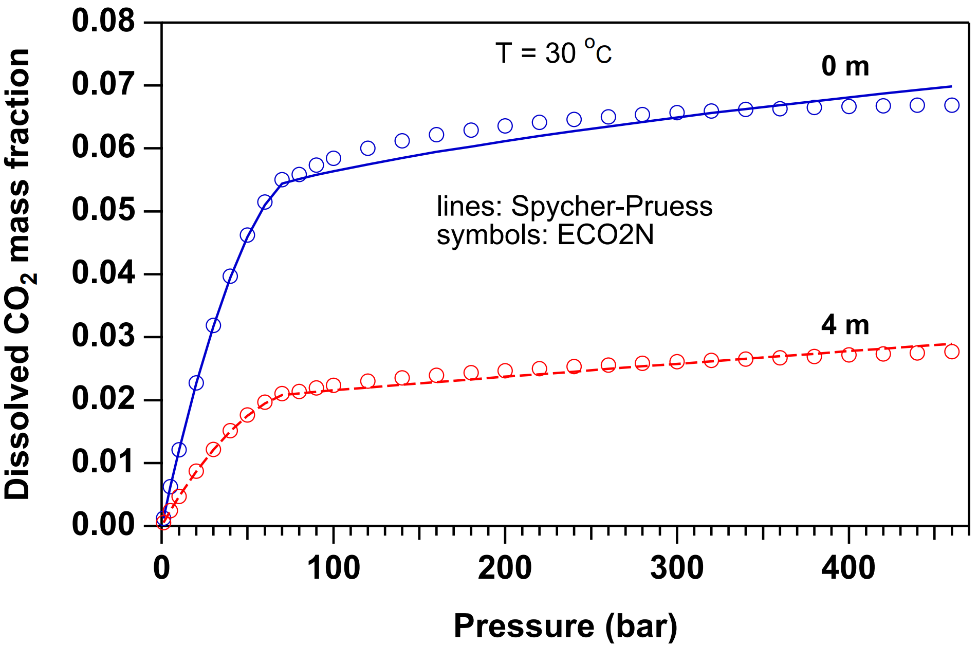
Figure 12 Dissolved CO₂ mass fractions in two-phase system at \(T\) = 30˚C for pure water (0m) and 4-molal NaCl brine. Lines represent the original correlation of Spycher & Pruess, 2005 that uses a Redlich-Kwong EOS for molar volume of CO₂. Symbols represent data calculated by ECO2N in which the molar volume of CO₂ is obtained from the correlations of Altunin, 1975.

Figure 13 H₂O mass fractions in gas in two-phase system at \(T\) = 30˚C for pure water (0m) and 4-molal NaCl brine. Lines represent the original correlation of Spycher & Pruess, 2005 that uses a Redlich-Kwong EOS for molar volume of CO₂. Symbols represent data calculated by ECO2N in which the molar volume of CO₂ is obtained from the correlations of Altunin, 1975.

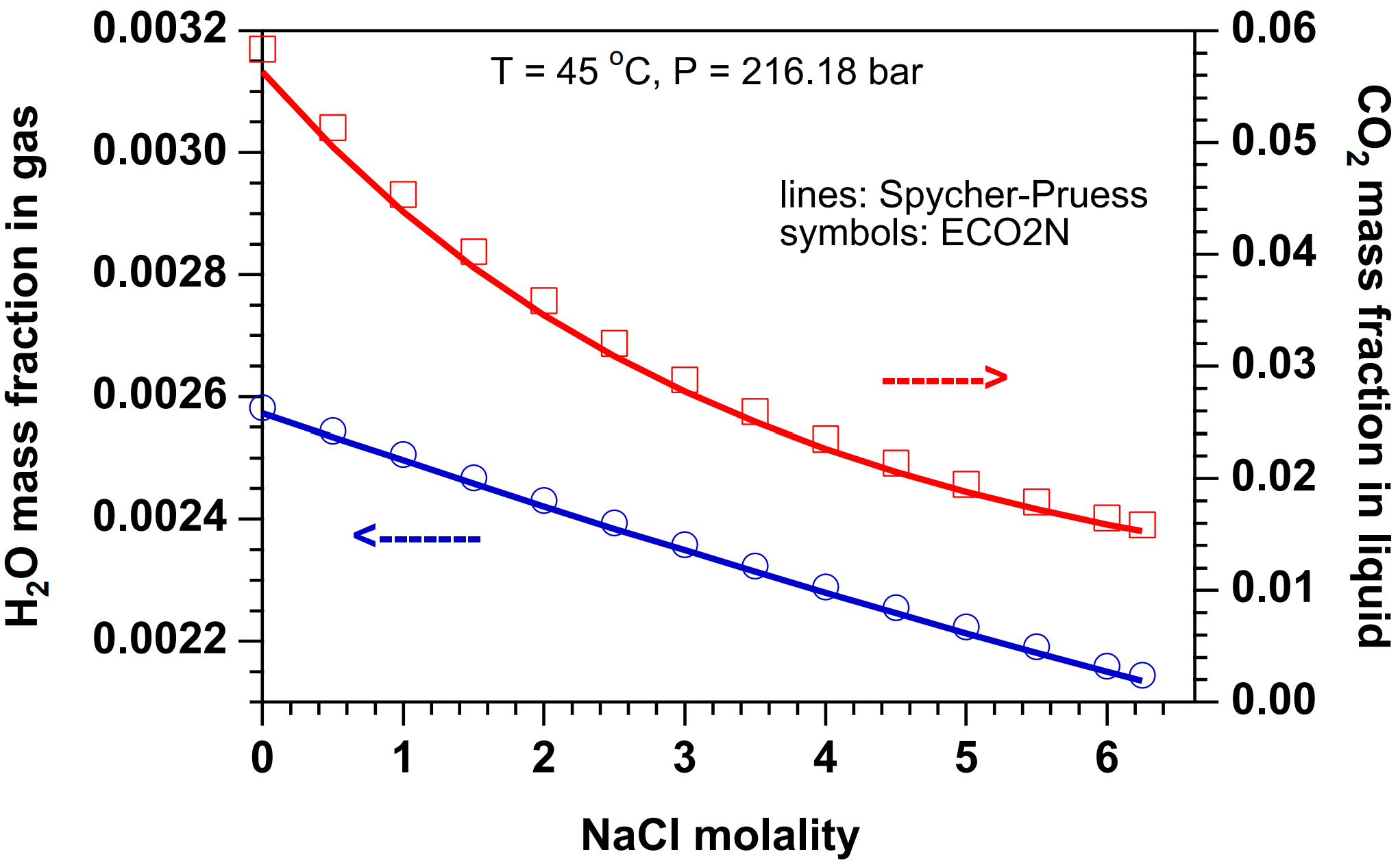
Figure 14 Concentration of water in gas and CO₂ in the liquid (aqueous) phase at (\(T\), \(P\)) = (45˚C, 216.18 bar), for salinities ranging from zero to fully saturated. Lines were calculated from the correlation of Spycher & Pruess, 2005 that uses a Redlich-Kwong EOS for molar volume of CO₂. Symbols represent data calculated by ECO2N from a modified correlation in which the molar volume of CO₂ is obtained from the correlations of Altunin, 1975.

For conditions of interest to geologic dispoal of CO₂, equilibrium between aqueous and gas phases corresponds to a dissolved CO₂ mass fraction in the aqueous phase, \(X_{2, eq}\), on the order of a few percent, while the mass fraction of water in the gas phase, \(Y_{1, eq}\), is a fraction of a percent, so that gas phase CO₂ mass fraction \(Y_{2, eq}\) = 1 - \(Y_{1, eq}\) is larger than 0.99. The relationship between CO₂ mass fraction \(X_3\) and phase composition of the fluid mixture is as follows (see Figure 15):

• \(X_3\) < \(X_{2, eq}\) corresponds to single-phase liquid conditions;

• \(X_3\) > \(X_{2, eq}\) corresponds to single-phase gas;

• intermediate values \(X_{2, eq}\) ≤ \(X_3\) ≤ \(Y_{2, eq}\) correspond to two-phase conditions with different proportions of aqueous and gas phases.

Dissolved NaCl concentrations may for typical sequestration conditions range as high as 6.25 molal. This corresponds to mass fractions of up to \(X_{sm}\) = 26.7% in the two-component system water-salt. Phase conditions as a function of \(X_{sm}\) are as follows:

• \(X_{sm}\) ≤ \(XEQ\) corresponds to dissolved salt only;

• \(X_{sm}\) > \(XEQ\) corresponds to conditions of a saturated NaCl brine and solid salt.

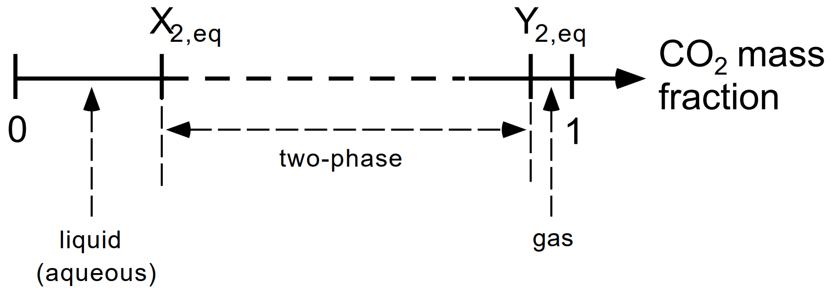
Figure 15 CO₂ phase partitioning in the system H₂O - NaCl - CO₂. The CO₂ mass fraction in brine-CO₂ mixtures can vary in the range from 0 (no CO₂) to 1 (no brine). \(X_{2, eq}\) and \(Y_{2, eq}\) denote, respectively, the CO₂ mass fractions in aqueous and gas phases corresponding to equilibrium phase partitioning in two-phase conditions. Mass fractions less than \(X_{2, eq}\) correspond to conditions in which only an aqueous phase is present, while mass fractions larger than \(Y_{2, eq}\) correspond to single-phase gas conditions. Mass fractions intermediate between \(X_{2, eq}\) and \(Y_{2, eq}\) correspond to two-phase conditions with different proportions of aqueous and gas phases.

Phase Change

In single-phase (aqueous or gas) conditions, the third primary variable X3 is the CO₂ mass fraction in that phase. In single-phase aqueous conditions, we must have \(X_3\) ≤ \(X_{2, eq}\), while in single-phase gas conditions, we must have \(X_3\) ≥ \(Y_{2, eq}\). The possibility of phase change is evaluated during a simulation by monitoring \(X_3\) in each grid block. The criteria for phase change from single-phase to two-phase conditions may be written as follow:

• single-phase aqueous conditions: a transition to two-phase conditions (evolution of a gas phase) will occur when \(X_3\) > \(X_{2, eq}\);

• single-phase gas conditions: a transition to two-phase conditions (evolution of an aqueous phase) will occur when \(X_3\) < \(Y_{2, eq}\) = 1 - \(Y_{1, eq}\).

When two-phase conditions evolve in a previously single-phase grid block, the third primary variable is switched to \(X_3\) = \(S_g\) + 10. If the transition occurred from single-phase liquid conditions, the starting value of \(S_g\) is chosen as 10^-6; if the transition occurred from single-phase gas, the starting value is chosen as 1 - 10^-6.

In two-phase conditions, the third primary variable is \(X_3\) = \(S_g\) + 10. For two-phase conditions to persist, \(X_3\) must remain in the range (10, 11 - \(S_s\)). Transitions to single-phase conditions are recognized as follows:

• if \(X_3\) < 10 (i.e., \(S_g\) < 0): gas phase disappears; make a transition to single-phase liquid conditions;

• if \(X_3\) > 11 - \(S_s\) (i.e., \(S_g\) > 1 - \(S_s\)): liquid phase disappears; make a transition to single-phase gas conditions.

Phase change involving (dis-)appearance of solid salt is recognized as follows. When no solid salt is present, the second primary variable \(X_{sm}\) is the concentration (mass fraction referred to total water plus salt) of dissolved salt in the aqueous phase. The possibility of precipitation starting is evaluated by comparing \(X_{sm}\) with \(XEQ\), the equilibrium solubility of NaCl at prevailing temperature. If \(X_{sm}\) ≤ \(XEQ\) no precipitation occurs, whereas for \(X_{sm}\) > \(XEQ\) precipitation starts. In the latter case, variable \(X_{sm}\) is switched to \(S_s\) + 10, where solid saturation \(S_s\) is initialized with a small non-zero value (10^-6). If a solid phase is present, the variable \(X_{sm}\) = \(S_s\) + 10 is monitored. Solid phase disappears if \(X_{sm}\) < 10, in which case primary variable \(X_{sm}\) is switched to salt concentration, and is initialized as slightly below saturation, \(X_{sm}\) = \(XEQ\) - 10^-6.

Conversion of Units

The Spycher & Pruess, 2005 model for phase partitioning in the system H₂O-NaCl-CO₂ is formulated in molar quantities (mole fractions and molalities), while TOUGH2/ECO2N describes phase compositions in terms of mass fractions. This section presents the equations and parameters needed for conversion between the two sets of units. The conversion between various concentration variables (mole fractions, molalities, mass fractions) does not depend upon whether or not concentrations correspond to equilibrium between liquid and gas phases; accordingly, the relations given below are valid regardless of the magnitude of concentrations.

Let us consider an aqueous phase with dissolved NaCl and CO₂. For a solution that is m-molal in NaCl and n-molal in CO₂, total mass per kg of water is

(77)\[M = 1000 (g H_2 O) + m M_{NaCl} (g NaCl) + n M_{CO_2} (g CO_2)\]

where \(M_{NaCl}\) and M_{CO_2} are the molecular weights of NaCl and CO₂, respectively (see Table 101). Assuming NaCl to be completely dissociated, the total moles per kg of water are

(78)\[m_T = \frac{1000}{M_{H_2 O}} + 2m + n\]

The Spycher & Pruess, 2005 correlations provide CO₂ mole fraction \(x_2\) in the aqueous phase and H₂O mole fraction \(y_1\) in the gas phase as functions of temperature, pressure, and salt concentration (molality). For a CO₂ mole fraction x2 we have \(n\) = \(x_2 m_T\) from which, using Eq. (78), we obtain

(79)\[n = \frac{x_2 \left( 2 m + \frac{1000}{M_{H_2 O}} \right)}{1 - x_2}\]

CO₂ mass fraction \(X_2\) in the aqueous phase is obtained by dividing the CO₂ mass in \(n\) moles by the total mass

(80)\[X_2 = \frac{n M_{CO_2}}{1000 + m M_{NaCl} + n M_{CO_2}}\]

Water mass fraction \(Y_1\) in the CO₂-rich phase is simply

(81)\[Y_1 = \frac{y1 M_{H_2 O}}{y1 M_{H_2 O} + \left( 1 - y_1 \right) M_{CO_2}}\]

The molecular weights of the various species are listed in Table 101 (Evans, 1982).

Table 101 Molecular weights in the system H₂O-NaCl-CO₂.

Species	Mol. weight
H2O	18.016
Na	22.991
Cl	35.457
NaCl	58.448
CO2	44.0

Thermophysical Properties of Water-NaCl-CO₂ Mixtures

Thermophysical properties needed to model the flow of water-salt-CO₂ mixtures in porous media include density, viscosity, and specific enthalpy of the fluid phases as functions of temperature, pressure, and composition, and partitioning of components among the fluid phases. Many of the needed parameters are obtained from the same correlations as were used in the EWASG property module of TOUGH2 (Battistelli et al., 1997). EWASG was developed for geothermal applications, and consequently considered conditions of elevated temperatures > 100˚C, and modest CO₂ partial pressures of order 1-10 bar. The present ECO2N module targets the opposite end of the temperature and pressure range, namely, modest temperatures below 110˚C, and high CO₂ pressures up to several hundred bar.

Water properties in TOUGH2/ECO2N are calculated, as in other members of the TOUGH family of codes, from the steam table equations as given by the International Formulation Committee (IFC, 1967). Properties of pure CO₂ are obtained from correlations developed by Altunin, 1975. We began using Altunin’s correlations in 1999 when a computer program implementingthem was conveniently made available to us by Victor Malkovsky of the Institute of Geology of Ore Deposits, Petrography, Mineralogy and Geochemistry (IGEM) of the Russian Academy of Sciences, Moscow. Altunin’s correlations were subsequently extensively cross-checked against experimental data and alternative PVT formulations, such as Span & Wagner, 1996. They were found to be very accurate ([Garcia, 2003]), so there is no need to change to a different formulation.

Altunin’s correlations are not used directly in the code, but are used ahead of a TOUGH2/ECO2N simulation to tabulate density, viscosity, and specific enthalpy of pure CO₂ on a regular grid of (\(T\), \(P\))-values. These tabular data are provided to the ECO2N module in a file called “CO2TAB”, and property values are obtained during the simulation by means of bivariate interpolation. Figure 16 shows the manner in which CO₂ properties are tabulated, intentionally showing a coarse (\(T\), \(P\))-grid so that pertinent features of the tabulation may be better seen. (For actual calculations, we use finer grid spacings; the CO2TAB data file distributed with ECO2N covers the range 3.04 ˚C ≤ \(T\) ≤ 103.04 ˚C with \(\Delta T\) = 2˚C and 1 bar ≤ \(P\) ≤ 600 bar with \(\Delta T\) ≤ 4 bar in most cases. The ECO2N distribution includes a utility program for generating CO2TAB files if users desire a different (\(T\), \(P\))-range or different increments). As shown in Figure 16, the tabulation is made in such a way that for sub-critical conditions the saturation line is given by diagonals of the interpolation quadrangles. On the saturation line, two sets of data are provided, for liquid and gaseous CO₂, respectively, and in quadrangles that include points on both sides of the saturation line, points on the “wrong” side are excluded from the interpolation. This scheme provides for an efficient and accurate determination of thermophysical properties of CO₂.

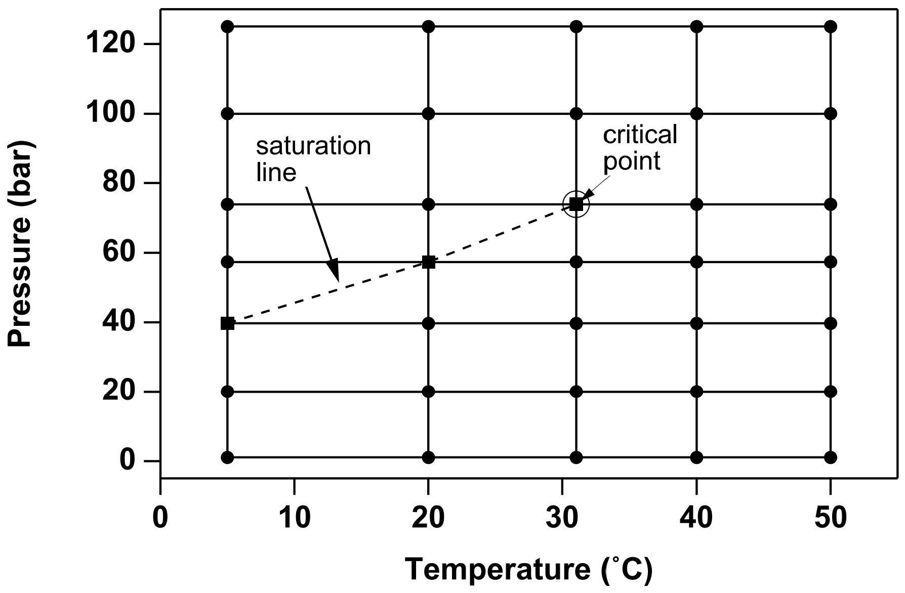
Figure 16 Schematic of the temperature-pressure tabulation of CO₂ properties. The saturation line (dashed) is given by the diagonals of interpolation rectangles.

An earlier version of ECO2N explicitly associated partial pressures of water (vapor) and CO₂ with the gas phase, and calculated CO₂ dissolution in the aqueous phase from the CO₂ partial pressure, using an extended version of Henry’s law (Pruess et al., 2002). The present version uses a methodology for calculating mutual solubilities of water and CO₂ (Spycher & Pruess, 2005) that is much more accurate, but has a drawback insofar as no partial pressures are associated with the individual fluid components. This makes it less straightforward to calculate thermophysical properties of the gas phase in terms of individual fluid components. We are primarily interested in the behavior of water-salt-CO₂ mixtures at moderate temperatures, \(T\) < 100˚C, say, where water vapor pressure is a negligibly small fraction of total pressure. Under these conditions the amount of water present in the CO₂-rich phase, henceforth referred to as “gas”, is small. Accordingly, we approximate density, viscosity, and specific enthalpy of the gas phase by the corresponding properties of pure CO₂, without water present.

Density

Brine density \(\rho_b\) for the binary system water-salt is calculated as in Battistelli et al., 1997 from the correlations of Haas, 1976 and Andersen et al., 1992. The calculation starts from aqueous phase density without salinity at vapor-saturated conditions, which is obtained from the correlations given by the International Formulation Committee (IFC, 1967). Corrections are then applied to account for effects of salinity and pressure. The density of aqueous phase with dissolved CO₂ is calculated assuming additivity of the volumes of brine and dissolved CO₂.

(82)\[\frac{1}{\rho_{aq}} = \frac{1 - X_2}{\rho_b} + \frac{X_2}{\rho_{CO_2}}\]

where \(X_2\) is the mass fraction of CO₂ in the aqueous phase. Partial density of dissolved CO₂, \(\rho_{CO_2}\), is calculated as a function of temperature from the correlation for molar volume of dissolved CO₂ at infinite dilution developed by Garcia, 2001.

(83)\[V_{\phi} = a + b T + c T^2 + d T^3\]

In Eq. (83), molar volume of CO₂ is in units of cm³ per gram-mole, temperature \(T\) is in ˚C, and \(a\), \(b\), \(c\), and \(d\) are fit parameters given in Table 102.

Table 102 Parameters for molar volume of dissolved CO₂ (83).

Parameter	Value
a	37.51
b	-9.585 × 10-2
c	8.740 × 10-4
d	-5.044 × 10-7

Partial density of dissolved CO₂ in units of kg/m³ is then

(84)\[\rho_{CO_2} = \frac{M_{CO_2}}{V_{\phi}} \times 10^{-3}\]

where \(M_{CO_2}\) = 44.0 is the molecular weight of CO₂.

Dissolved CO₂ amounts at most to a few percent of total aqueous density. Accordingly, dissolved CO₂ is always dilute, regardless of total fluid pressure. It is then permissible to neglect the pressure dependence of partial density of dissolved CO₂, and to use the density corresponding to infinite dilution.

As had been mentioned above, the density of the CO₂-rich (gas) phase is obtained by neglecting effects of water, and approximating the density by that of pure CO₂ at the same temperature and pressure conditions. Density is obtained through bivariate interpolation from a tabulation of CO₂ densities as function of temperature and pressure, that is based on the correlations developed by Altunin, 1975.

Viscosity

Brine viscosity is obtained as in EWASG from a correlation presented by Phillips, 1981, that reproduces experimental data in the temperature range from 10-350˚C for salinities up to 5 molal and pressures up to 500 bar within 2%. No allowance is made for dependence of brine viscosity on the concentration of dissolved CO₂. Viscosity of the CO₂-rich phase is approximated as being equal to pure CO₂, and is obtained through tabular interpolation from the correlations of Altunin, 1975.

Specific Enthalpy

Specific enthalpy of brine is calculated from the correlations developed by Lorenz et al., 2000, which are valid for all salt concentrations in the temperature range from 25˚C ≤ \(T\) ≤ 300˚C. The enthalpy of aqueous phase with dissolved CO₂ is obtained by adding the enthalpies of the CO₂ and brine (pseudo-) components, and accounting for the enthalpy of dissolution of CO₂.

(85)\[h_{aq} = \left( 1 - X_2 \right) h_b + X_2 h_{CO_2, aq}\]

\(h_{CO_2, aq} = h_{CO_2} + h_{dis}\) is the specific enthalpy of aqueous (dissolved) CO₂, which includes heat of dissolution effects that are a function of temperature and salinity. For gas-like (low pressure) CO₂, the specific enthalpy of dissolved CO₂ is

(86)\[h_{CO_2, aq} (T, P, X_s) = h_{CO_2, g} (T, P) + h_{dis, g} (T, X_s)\]

where \(h_{dis, g}\) is obtained as in Battistelli et al., 1997 from an equation due to Himmelblau, 1959. For geologic sequestration we are primarily interested in liquid-like (high-pressure) CO₂, for which the specific enthalpy of dissolved CO₂ may be written

(87)\[h_{CO_2, aq} (T, P, X_s) = h_{CO_2, l} (T, P) + h_{dis, l} (T, X_s)\]

Here \(h_{dis, l}\) is the specific heat of dissolution for liquid-like CO₂. Along the CO₂ saturation line, liquid and gaseous CO₂ phases may co-exist, and the expressions Eqs. (86) and (87) must be equal there. We obtain

(88)\[h_{dis, l} (T, X_s) = h_{dis, g} (T, X_s) + h_{CO_2, gl} (T)\]

where \(h_{CO_2, gl} (T) = h_{CO_2, g} (T, P_s) - h_{CO_2, l} (T, P_s)\) is the specific enthalpy of vaporization of CO₂, and \(P_s = P_s (T)\) is the saturated vapor pressure of CO₂ at temperature \(T\). Depending upon whether CO₂ is in gas or liquid conditions, we use Eq. (86) or (87) in Eq. (85) to calculate the specific enthalpy of dissolved CO₂. At the temperatures of interest here, \(h_{dis, g}\) is a negative quantity, so that dissolution of low-pressure CO₂ is accompanied by an increase in temperature. \(h_{CO_2, gl}\) is a positive quantity, which will reduce or cancel out the heat-of-dissolution effects. This indicates that dissolution of liquid CO₂ will produce less temperature increase than dissolution of gaseous CO₂, and may even cause a temperature decline if \(h_{CO_2, gl}\) is sufficiently large.

Application of Eq. (85) is straightforward for single-phase gas and two-phase conditions, where \(h_{CO_2}\) is obtained as a function of temperature and pressure through bivariate interpolation from a tabulation of Altunin’s correlation (Altunin, 1975). A complication arises in evaluating \(h_{CO_2}\) for single-phase aqueous conditions. We make the assumption that \(h_{CO_2} (P, X_s, X_2, T)\) for single-phase liquid is identical to the value in a two-phase system with the same composition of the aqueous phase. To determine \(h_{CO_2}\), it is then necessary to invert the Spycher & Pruess, 2005 phase partitioning relation \(X_2 = X_2 (P, T, X_s)\), in order to obtain the pressure \(P\) in a two-phase aqueous-gas system that would correspond to a dissolved CO₂ mass fraction \(X_2\) in the aqueous phase, \(P = P(X_2, X_s, T)\). The inversion is accomplished by Newtonian iteration, using a starting guess \(P_0\) for \(P\) that is obtained from Henry’s law. Specific enthalpy of gaseous CO₂ in the two-phase system is then calculated as \(h_{CO_2} = h_{CO_2} (T, P)\), and specific enthalpy of dissolved CO₂ is \(h_{CO_2} + h_{dis}\).

Description

Initialization Choices

Flow problems in TOUGH2/ECO2N will generally be initialized with the primary thermodynamic variables as used in the code, but some additional choices are available for the convenience of users. The internally used variables are (\(P\), \(X_{sm}\), \(X_3\), \(T\)) for grid blocks in single-phase (liquid or gas) conditions and (\(P\), \(X_{sm}\), \(S_g\) + 10, \(T\)) for two-phase (liquid and gas) grid blocks (see Table 100). Here \(X_3\) is the mass fraction of CO₂ in the fluid. As had been discussed above, for conditions of interest to geologic sequestration of CO₂, \(X_3\) is restricted to small values 0 ≤ \(X_3\) ≤ \(X_{2, eq}\) (a few percent) for single-phase liquid conditions, or to values near 1 (\(Y_{2, eq}\) ≤ \(X_3\) ≤ 1, with \(Y_{2, eq}\) > 0.99 typically) for single-phase gas (Figure 15). Intermediate values \(X_{2, eq}\) < \(X_3\) < \(Y_{2, eq}\) correspond to two-phase conditions, and thus should be initialized by specifying \(S_g\) + 10 as third primary variable. As a convenience to users, ECO2N allows initial conditions to be specified in the full range 0 ≤ \(X_3\) ≤ 1. During the initialization phase of a simulation, a check is made whether \(X_3\) is in fact within the range of mass fractions that correspond to single-phase (liquid or gas) conditions. If this is found not to be the case, the conditions are recognized as being two-phase, and the corresponding gas saturation is calculated from the phase equilibrium constraint.

(89)\[X_3 \left( S_l \rho_l + S_g \rho_g \right) = S_l \rho_l X_{2, eq} + S_g \rho_g Y_{2, eq}\]

Using \(S_l = 1 - S_g - S_s\), with Ss the “solid saturation” (fraction of pore space occupied by solid salt), we obtain

(90)\[S_g = A \left( 1 - S_s \right)\]

and the third primary variable is reset internally to \(X_3\) = \(S_g\) + 10. Here the parameter \(A\) is given by

(91)\[A = \frac{\left( X_3 - X_{2, eq} \right) \rho_l}{\left( X_3 - X_{2, eq} \right) \rho_l + \left( Y_{2, eq} - X_3 \right) \rho_g}\]

Users may think of specifying single-phase liquid (aqueous) conditions by setting \(X_3\) = 10 (corresponding to \(S_g\) = 0), and single-phase gas conditions by setting \(X_3\) = 11 - \(S_s\) (corresponding to \(Sl\) = 0). Strictly speaking this is not permissible, because two-phase initialization requires that both \(S_g\) > 0 and \(S_l\) > 0. Single-phase states should instead be initialized by specifying primary variable \(X_3\) as CO₂ mass fraction. However, as a user convenience, ECO2N accepts initialization of single-phase liquid conditions by specifying \(X_3\) = 10 (\(S_g\) = 0). Such specification will be converted internally to two-phase in the initialization phase by adding a small number (10^-11) to the third primary variable, changing conditions to two-phase with a small gas saturation \(S_g\) = 10^-11.

Salt concentration or saturation of solid salt, if present, is characterized in ECO2N by means of the second primary variable \(X_{sm}\). When no solid phase is present, \(X_{sm}\) denotes \(X_s\), the mass fraction of NaCl referred to the two-component system water-NaCl. This is restricted to the range 0 ≤ \(X_{sm}\) ≤ \(XEQ\), where \(XEQ = XEQ(T)\) is the solubility of salt. For \(X_{sm}\) > 10 this variable means \(S_s\) + 10, solid saturation plus 10. Users also have the option to specify salt concentration by means of molality \(m\) by assigning \(X_{sm} = -m\). Such specification will in the initialization phase be internally converted to \(X_s\) by using Eq. (75). When salt concentration (as a fraction of total H₂O + NaCl mass) exceeds \(XEQ\), this corresponds to conditions in which solid salt will be present in addition to dissolved salt in the aqueous phase. Such states should be initialized with a second primary variable \(X_{sm}\) = \(S_s\) + 10. However, ECO2N accepts initialization with \(X_{sm}\) > \(XEQ\), recognizes this as corresponding to presence of solid salt, and converts the second primary variable internally to the appropriate solid saturation that will result in total salt mass fraction in the binary system water-salt being equal to \(X_{sm}\). The conversion starts from the following equation.

(92)\[X_{sm} = \frac{XEQ \times S_l \rho_l \left( 1 - X_2 \right) + S_s \rho_s}{S_l \rho_l \left( 1 - X_2 \right) + S_s \rho_s}\]

where the numerator gives the total salt mass per unit volume, in liquid and solid phases, while the denominator gives the total mass of salt plus water. Substituting \(S_l = 1 - S_g - S_s\), this can be solved for \(S_s\) to yield

(93)\[S_s = \frac{B \left( 1 - S_g \right)}{1 + B}\]

where the parameter \(B\) is given by

(94)\[B = \frac{\left( X_{sm} - XEQ \right) \rho_l \left( 1 - X_2 \right)}{\rho_s \left( 1 - X_{sm} \right)}\]

The most general conditions arise when both the second and third primary variables are initialized as mass fractions, nominally corresponding to single-phase fluid conditions with no solid phase present, but both mass fractions being in the range corresponding to two-phase fluid conditions with precipitated salt. Under these conditions, Eqs. (90) and (93) are solved simultaneously in ECO2N for \(S_s\) and \(S_g\), yielding

(95)\[S_g = \frac{A}{1 + B - A \times B}\]

(96)\[S_s = \frac{B \times \left( 1 - A \right)}{1 + B - A \times B}\]

Then both second and third primary variables are converted to phase saturations, \(S_s\) + 10 and \(S_g\) + 10, respectively.

Permeability Change from Precipitation and Dissolution of Salt

ECO2N offers several choices for the functional dependence of relative change in permeability, \(\frac{k}{k_0}\), on relative change in active flow porosity.

(97)\[\frac{k}{k_0} = f \left( \frac{\phi_f}{\phi_0} \right) \equiv f \left( 1 - S_s \right)\]

The simplest model that can capture the converging-diverging nature of natural pore channels consists of alternating segments of capillary tubes with larger and smaller radii, respectively; see Figure 17. While in straight capillary tube models permeability remains finite as long as porosity is non-zero, in models of tubes with different radii in series, permeability is reduced to zero at a finite porosity.

Conceptual model

Tubes-in-series

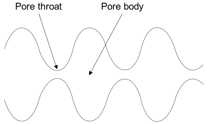
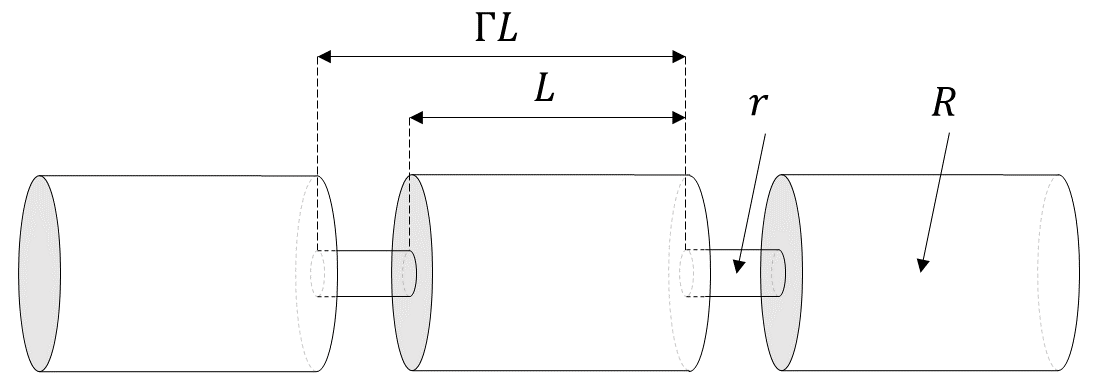
Figure 17 Model for converging-diverging pore channels.

From the tubes-in-series model shown in Figure 17, the following relationship can be derived (Verma & Pruess, 1988)

(98)\[\frac{k}{k_0} = \theta^2 \frac{1 - \Gamma + \frac{\Gamma}{\omega^2}}{1 - \Gamma + \Gamma \left( \frac{\theta}{\theta + \omega - 1} \right)^2}\]

Here

(99)\[\theta = \frac{1 - S_s - \phi_r}{1 - \phi_r}\]

depends on the fraction \(1 - S_s\) of original pore space that remains available to fluids, and on a parameter \(\phi_r\), which denotes the fraction of original porosity at which permeability is reduced to zero. \(\Gamma\) is the fractional length of the pore bodies, and the parameter \(\omega\) is given by

(100)\[\omega = 1 + \frac{\frac{1}{\Gamma}}{\frac{1}{\phi_r} - 1}\]

Therefore, Eq. (98) has only two independent geometric parameters that need to be specified, \(\phi_r\) and \(\Gamma\). As an example, Figure 18 shows the permeability reduction factor from Eq. (98), plotted against \(\frac{\phi}{\phi_0} \equiv \left( 1 - S_s \right)\), for parameters of \(\phi_r\) = \(\Gamma\) = 0.8.

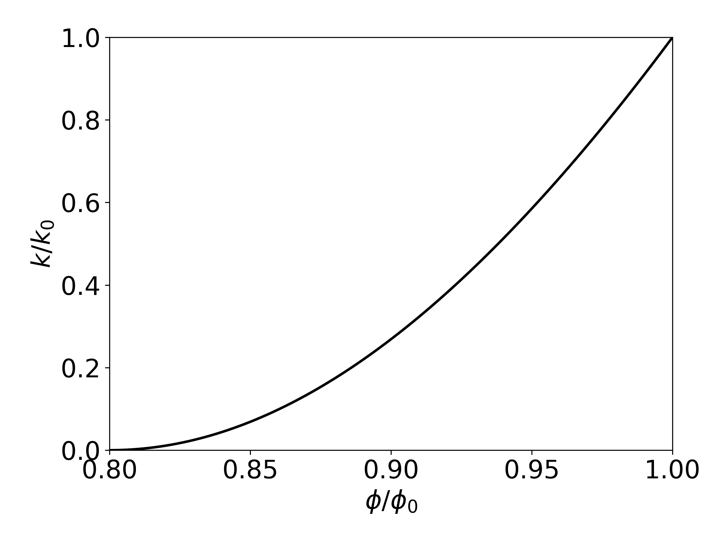
Figure 18 Porosity-permeability relationship for tubes-in-series model, after Verma & Pruess, 1988.

For parallel-plate fracture segments of different aperture in series, a relationship similar to Eq. (98) is obtained, the only difference being that the exponent 2 is replaced everywhere by 3 (Verma & Pruess, 1988). If only straight capillary tubes of uniform radius are considered, we have \(\phi_r\) = 0, \(\Gamma\) = 0, and Eq. (71) simplifies to

(101)\[\frac{k}{k_0} = \left( 1 - S_s \right)^2\]

Selections

Various options for ECO2N can be selected through parameter specifications in data block SELEC. Default choices corresponding to various selection parameters set equal to zero provide the most comprehensive thermophysical property model. Certain functional dependencies can be turned off or replaced by simpler and less accurate models, see below. These options are offered to enable users to identify the role of different effects in a flow problem, and to facilitate comparison with other simulation programs that may not include full dependencies of thermophysical properties.

Table 103 Record SELEC.1.

Parameter	Format	Description
IE(1)	I5	set equal to 1, to read one additional data record (a larger value with more data records is acceptable, but only one additional record will be used by ECO2N).
IE(11)	I5	selects dependence of permeability on the fraction \(\frac{\phi_f}{\phi_0} = \left( 1 - S_s \right)\) of original pore space that remains available to fluids: 0: permeability does not vary with \(\phi_f\). 1: \(\frac{k}{k_0} = \left( 1 - S_s \right)^{\gamma}\), with \(\gamma\) = FE(1). 2: fractures in series, i.e., Eq. (98) with exponent 2 everywhere replaced by 3. 3: tubes-in-series, i.e., Eq. (98).
IE(12)	I5	allows choice of model for water solubility in CO2: 0: after Spycher and Pruess (2005). 1: evaporation model; i.e., water density in the CO2-rich phase is calculated as density of saturated water vapor at prevailing temperature and salinity.
IE(13)	I5	allows choice of dependence of brine density on dissolved CO2: 0: brine density varies with dissolved CO2 concentration, according to García’s (2001) correlation for temperature dependence of molar volume of dissolved CO2. 1: brine density is independent of CO2 concentration.
IE(14)	I5	allows choice of treatment of thermophysical properties as a function of salinity: 0: full dependence. 1: no salinity dependence of thermophysical properties (except for brine enthalpy; salt solubility constraints are maintained).
IE(15)	I5	allows choice of correlation for brine enthalpy at saturated vapor pressure: 0: after Lorenz et al. (2000). 1: after Michaelides (1981). 2: after Miller (1978).

Table 104 Record SELEC.2.

Parameter	Format	Description
FE(1)	E10.4	parameter \(\gamma\) (for IE(11) = 1); parameter \(\phi_r\) (for IE(11) = 2, 3).
FE(2)	E10.4	parameter \(\Gamma\) (for IE(11) = 2, 3).