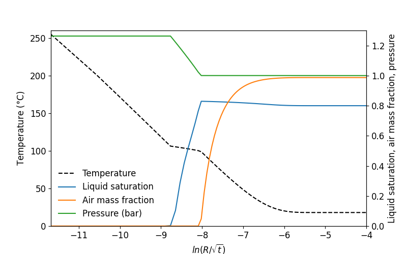
Plot profiles

The objective of this example is to import the output results and plot the profiles of temperature, pressure, liquid saturation and air mass fraction.

Here, we assume that the simulation’s output have been written in the file “OUTPUT”. To import the results, we use the function toughio.read_output(). The variable outputs is a list with three toughio.Output corresponding to the three time steps requested in the preprocessing example. In this example, we want to look at the last time step (index -1).

import numpy as np
import toughio

outputs = toughio.read_output("OUTPUT")
output = outputs[-1]

t = output.data["T"]
p = output.data["P"]
sl = output.data["SL"]
xm = output.data["XAIRG"]

It is well known that for the stated conditions (1-D radial geometry, homogeneous medium, uniform initial conditions, and a constant-rate line source) the problem has a similarity solution: The partial differential equations for this complex two-phase flow problem can be rigorously transformed into a set of ordinary differential equations in the variable \(Z = R/\sqrt{t}\), which can be easily solved to any degree of accuracy desired by means of one-dimensional numerical integration (O’Sullivan, 1981). Comparison of TOUGH2 simulations with the semi-analytical similarity solution has shown excellent agreement (Doughty and Pruess, 1992). To define such variable, we first need to import the mesh

mesh = toughio.read_mesh("mesh.pickle")
R = np.log(mesh.centers[:, 0] / (output.time) ** 0.5)

Now that the required data have been imported, we can plot the results using matplotlib.

import matplotlib.pyplot as plt
plt.rc("font", size=12)

fig, ax1 = plt.subplots(figsize=(8, 5))
ax2 = ax1.twinx()

ax1.plot(R, t, color="black", linestyle="--", label="Temperature")
ax1.set_ylim(0.0, 260.0)
ax1.set_ylabel("Temperature ($\degree$C)")

ax2.plot(R, sl, label="Liquid saturation")
ax2.plot(R, xm, label="Air mass fraction")
ax2.plot(R, p * 1.0e-5, label="Pressure (bar)")
ax2.set_ylim(0.0, 1.3)
ax2.set_ylabel("Liquid saturation, air mass fraction, pressure")

ax1.set_xlim(R.min(), -4.0)
ax1.set_xlabel("$ln(R/\sqrt{t})$")

fig.legend(
    loc="lower left",
    bbox_to_anchor=(0.0, 0.0),
    bbox_transform=ax1.transAxes,
    frameon=False,
)

<matplotlib.legend.Legend object at 0x7fda2dcb9a60>