Generate mesh in Python with Gmsh

This examples describes how to generate a mesh using Gmsh in Python. It requires pygmsh v7 to be installed:

pip install pygmsh --user

The mesh can also be generated from scratch directly in Gmsh either using its GUI and/or its internal scripting language.

Note that toughio is not required at this preliminary stage of the pre-processing. This example only intends to show how the mesh used in this sample problem has been generated. The user is free to use any meshing software as long as the mesh format is supported by toughio (through meshio).

First, we import numpy and pygmsh.

import numpy as np
import pygmsh

We can define a bunch of useful variables such as the characteristic length or some parameters to characterize the model.

lc = 100.0                       # Characteristic length of mesh
xmin, xmax = 0.0, 2000.0         # X axis boundaries
zmin, zmax = -500.0, -2500.0     # Z axis boundaries

inj_z = -1500.0                  # Depth of injection
flt_offset = 50.0                # Offset of fault
flt_thick = 10.0                 # Thickness of fault
tana = np.tan(np.deg2rad(80.0))  # Tangeant of dipping angle of fault
dist = 500.0 - 0.5 * flt_thick   # Distance from injection point (0.0, -1500.0) to left wall of fault

bnd_thick = 10.0                 # Thickness of boundary elements

We start by defining the geometrical entity representing the fault. The fault is represented as a finite-thickness element that intersects all the layers of the model. To ensure conformity of the final mesh, each wall of the fault is represented by a segmented line where the positions of the nodes correspond to the intersections of the hanging (left) and foot (right) walls with the different layers. Note that the foot wall is inverted so that the fault entity forms a closed rectangular loop.

depths = [zmin, -1300.0, -1450.0, -1550.0, -1700.0, zmax]
fault_left = [[dist + (z - inj_z) / tana, z, 0.0] for z in depths]

depths = [zmin, -1300.0 + flt_offset, -1450.0 + flt_offset, -1550.0 + flt_offset, -1700.0 + flt_offset, zmax]
fault_right = [[dist + (z - inj_z) / tana + flt_thick, z, 0.0] for z in depths]

fault_pts = fault_left + fault_right[::-1]

Now, we define the aquifer located at the left side of the fault.

cenaq_left_pts = [
    [xmin, -1450.0, 0.0],
    [dist + (-1450.0 - inj_z) / tana, -1450.0, 0.0],
    [dist + (-1550.0 - inj_z) / tana, -1550.0, 0.0],
    [xmin, -1550.0, 0.0],
]
capro_top_left_pts = [
    [xmin, -1300.0, 0.0],
    [dist + (-1300.0 - inj_z) / tana, -1300.0, 0.0],
    [dist + (-1450.0 - inj_z) / tana, -1450.0, 0.0],
    [xmin, -1450.0, 0.0],
]
capro_bot_left_pts = [
    [xmin, -1550.0, 0.0],
    [dist + (-1550.0 - inj_z) / tana, -1550.0, 0.0],
    [dist + (-1700.0 - inj_z) / tana, -1700.0, 0.0],
    [xmin, -1700.0, 0.0],
]
uppaq_left_pts = [
    [xmin, zmin, 0.0],
    [dist + (zmin - inj_z) / tana, zmin, 0.0],
    [dist + (-1300.0 - inj_z) / tana, -1300.0, 0.0],
    [xmin, -1300.0, 0.0],
]
basaq_left_pts = [
    [xmin, -1700.0, 0.0],
    [dist + (-1700.0 - inj_z) / tana, -1700.0, 0.0],
    [dist + (zmax - inj_z) / tana, zmax, 0.0],
    [xmin, zmax, 0.0],
]

Likewise, we also define the aquifer located at the right side of the fault.

cenaq_right_pts = [
    [dist + (-1450.0 - inj_z + flt_offset) / tana + flt_thick, -1450.0 + flt_offset, 0.0],
    [xmax, -1450.0 + flt_offset, 0.0],
    [xmax, -1550.0 + flt_offset, 0.0],
    [dist + (-1550.0 - inj_z + flt_offset) / tana + flt_thick, -1550.0 + flt_offset, 0.0],
]
capro_top_right_pts = [
    [dist + (-1300.0 - inj_z + flt_offset) / tana + flt_thick, -1300.0 + flt_offset, 0.0],
    [xmax, -1300.0 + flt_offset, 0.0],
    [xmax, -1450.0 + flt_offset, 0.0],
    [dist + (-1450.0 - inj_z + flt_offset) / tana + flt_thick, -1450.0 + flt_offset, 0.0],
]
capro_bot_right_pts = [
    [dist + (-1550.0 - inj_z + flt_offset) / tana + flt_thick, -1550.0 + flt_offset, 0.0],
    [xmax, -1550.0 + flt_offset, 0.0],
    [xmax, -1700.0 + flt_offset, 0.0],
    [dist + (-1700.0 - inj_z + flt_offset) / tana + flt_thick, -1700.0 + flt_offset, 0.0],
]
uppaq_right_pts = [
    [dist + (zmin - inj_z) / tana + flt_thick, zmin, 0.0],
    [xmax, zmin, 0.0],
    [xmax, -1300.0 + flt_offset, 0.0],
    [dist + (-1300.0 - inj_z + flt_offset) / tana + flt_thick, -1300.0 + flt_offset, 0.0],
]
basaq_right_pts = [
    [dist + (-1700.0 - inj_z + flt_offset) / tana + flt_thick, -1700.0 + flt_offset, 0.0],
    [xmax, -1700.0 + flt_offset, 0.0],
    [xmax, zmax, 0.0],
    [dist + (zmax-inj_z) / tana + flt_thick, zmax, 0.0],
]

Then, we define the boundary elements. In this sample problem, a no-flow boundary condition is imposed on the left side of the model (default in TOUGH), and Dirichlet boundary conditions are imposed elsewhere. Thus, physical boundary elements must be defined at the top, right and bottom sides of the model. Similarly to the fault entity, boundary entities are segmented to ensure conformity of the final mesh.

bound_right_pts = [
    [xmax, zmin, 0.0],
    [xmax + bnd_thick, zmin, 0.0],
    [xmax + bnd_thick, zmax, 0.0],
    [xmax, zmax, 0.0],
    [xmax, -1700.0 + flt_offset, 0.0],
    [xmax, -1550.0 + flt_offset, 0.0],
    [xmax, -1450.0 + flt_offset, 0.0],
    [xmax, -1300.0 + flt_offset, 0.0],
]
bound_top_pts = [
    [xmin, zmin, 0.0],
    [dist + (zmin - inj_z) / tana, zmin, 0.0],
    [dist + (zmin - inj_z) / tana + flt_thick, zmin, 0.0],
    [xmax, zmin, 0.0],
    [xmax + bnd_thick, zmin, 0.0],
    [xmax + bnd_thick, zmin + bnd_thick, 0.0],
    [dist + (zmin - inj_z + bnd_thick) / tana + flt_thick, zmin + bnd_thick, 0.0],
    [dist + (zmin - inj_z + bnd_thick) / tana, zmin + bnd_thick, 0.0],
    [xmin, zmin + bnd_thick, 0.0],
]
bound_bot_pts = [
    [xmin, zmax, 0.0],
    [dist + (zmax - inj_z) / tana, zmax, 0.0],
    [dist + (zmax - inj_z) / tana + flt_thick, zmax, 0.0],
    [xmax, zmax, 0.0],
    [xmax + bnd_thick, zmax, 0.0],
    [xmax + bnd_thick, zmax - bnd_thick, 0.0],
    [dist + (zmax - inj_z - bnd_thick) / tana + flt_thick, zmax - bnd_thick, 0.0],
    [dist + (zmax - inj_z - bnd_thick) / tana, zmax - bnd_thick, 0.0],
    [xmin, zmax - bnd_thick, 0.0],
]

Once all the points have been created, we can now generate the geometry, assign rock types/materials as Gmsh physical properties, and generate the mesh. To refine the mesh in the injection zone, the characteristic length of each layer entity is increased the farther we get from the injection point. Note that layers are defined such that their characteristic lengths are increasing. This is because Gmsh keeps the first node defined in the geometry in case it detects duplicated nodes.

with pygmsh.geo.Geometry() as geo:
    # Define polygons
    fault = geo.add_polygon(fault_pts, mesh_size=0.1 * lc)
    cenaq_left = geo.add_polygon(cenaq_left_pts, mesh_size=0.1 * lc)
    capro_top_left = geo.add_polygon(capro_top_left_pts, mesh_size=0.2 * lc)
    capro_bot_left = geo.add_polygon(capro_bot_left_pts, mesh_size=0.2 * lc)
    uppaq_left = geo.add_polygon(uppaq_left_pts, mesh_size=2.0 * lc)
    basaq_left = geo.add_polygon(basaq_left_pts, mesh_size=2.0 * lc)
    cenaq_right = geo.add_polygon(cenaq_right_pts, mesh_size=0.75 * lc)
    capro_top_right = geo.add_polygon(capro_top_right_pts, mesh_size=0.75 * lc)
    capro_bot_right = geo.add_polygon(capro_bot_right_pts, mesh_size=0.75 * lc)
    uppaq_right = geo.add_polygon(uppaq_right_pts, mesh_size=2.0 * lc)
    basaq_right = geo.add_polygon(basaq_right_pts, mesh_size=2.0 * lc)
    bound_right = geo.add_polygon(bound_right_pts, mesh_size=lc)
    bound_top = geo.add_polygon(bound_top_pts, mesh_size=lc)
    bound_bot = geo.add_polygon(bound_bot_pts, mesh_size=lc)

    # Define materials
    geo.add_physical([uppaq_left, uppaq_right], "UPPAQ")
    geo.add_physical([capro_top_left, capro_bot_left, capro_top_right, capro_bot_right], "CAPRO")
    geo.add_physical([cenaq_left, cenaq_right], "CENAQ")
    geo.add_physical([basaq_left, basaq_right], "BASAQ")
    geo.add_physical(fault, "FAULT")
    geo.add_physical([bound_right, bound_top, bound_bot], "BOUND")

    # Remove duplicate entities
    geo.env.removeAllDuplicates()
    mesh = geo.generate_mesh(dim=2, algorithm=6)

    # Convert cell sets to material
    cell_data = [np.empty(len(c.data), dtype=int) for c in mesh.cells]
    field_data = {}
    for i, (k, v) in enumerate(mesh.cell_sets.items()):
        if k:
            field_data[k] = np.array([i + 1, 3])
            for ii, vv in enumerate(v):
                cell_data[ii][vv] = i + 1
    mesh.cell_data["material"] = cell_data
    mesh.field_data.update(field_data)
    mesh.cell_sets = {}

    # Remove lower dimension entities
    idx = [i for i, cell in enumerate(mesh.cells) if cell.type == "triangle"]
    mesh.cells = [mesh.cells[i] for i in idx]
    mesh.cell_data = {k: [v[i] for i in idx] for k, v in mesh.cell_data.items()}

    # Export the mesh for post-processing
    mesh.write("mesh.vtu")

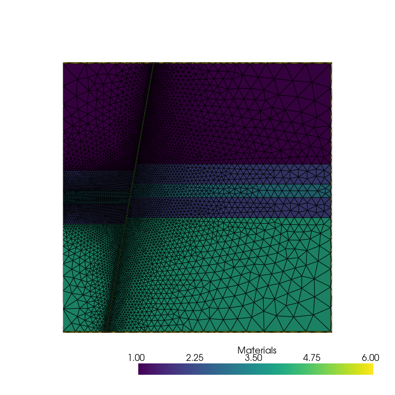
The generated mesh can be visualized in Python with pyvista.

import pyvista
pyvista.set_plot_theme("document")

p = pyvista.Plotter(window_size=(800, 800))
p.add_mesh(
    mesh=pyvista.from_meshio(mesh),
    scalar_bar_args={"title": "Materials"},
    show_scalar_bar=True,
    show_edges=True,
)
p.view_xy()
p.show()