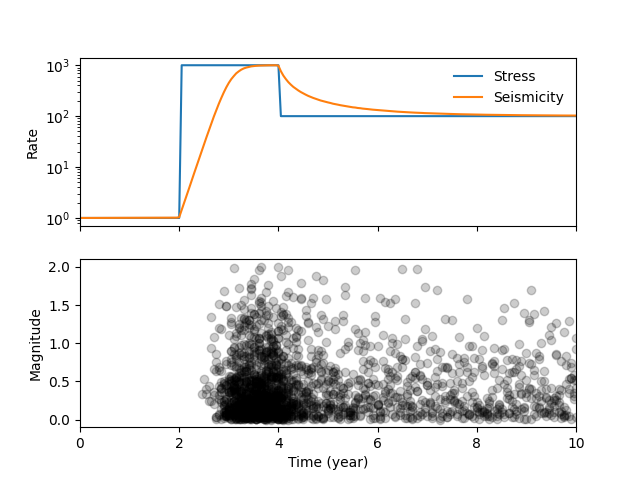
Modeling of seismicity

This example shows how to translate stressing rate to seismicity rate using the function bruces.modeling.seismicity_rate(). Modeled seismicity rate can then be used to generate a magnitude-time distribution using the function bruces.modeling.magnitude_time().

This example starts by generating a synthetic stressing rate with an instantaneous 1000 fold increase after 2 years followed by a 10 fold decrease after another 2 years.

The free parameter \(a \sigma\) of the rate-and-state model is arbitrarily set to 0.15. Note that bruces.modeling.seismicity_rate() outputs the seismicity rate \(r\) relative to the background seismicity rate \(r_0\). Modeling the magnitude-time distribution requires the actual seismicity rate \(r \times r_0\). Here, we assume that \(r_0\) = 1 event/year.

(0.0, 10.0)

import bruces
import numpy as np
import matplotlib.pyplot as plt

# Define stressing rate
stress_ini = 1.0e-3
times = np.linspace(0.0, 10.0, 201)
stress = np.ones(201) * stress_ini
stress[times > 2.0] = stress_ini * 1.0e3
stress[times > 4.0] = stress_ini * 1.0e2

# Model relative seismicity rate
rates = bruces.modeling.seismicity_rate(
    times=times,
    stress=stress,
    stress_ini=stress_ini,
    asigma=0.15,
)

# Model magnitude-time distribution
magnitudes = bruces.modeling.magnitude_time(
    times=times,
    rates=rates,
    m_bounds=[0.0, 2.0],
    seed=0,
)

# Plot
fig, ax = plt.subplots(2, 1, sharex=True)

ax[0].semilogy(times, stress / stress_ini, label="Stress")
ax[0].semilogy(times, rates, label="Seismicity")
ax[0].set_ylabel("Rate")
ax[0].legend(frameon=False)

for t, m in zip(times, magnitudes):
    if len(m):
        ax[1].scatter([t] * len(m), m, color="black", alpha=0.2)

ax[1].set_xlabel("Time (year)")
ax[1].set_ylabel("Magnitude")
ax[1].set_xlim(times.min(), times.max())